Ray Optics Module

Simulate Ray Tracing in Optically Large Systems

The Ray Optics Module is an add-on to the COMSOL Multiphysics® software that allows you to model electromagnetic wave propagation with a ray-tracing approach. The propagating waves are treated as rays that can be reflected, refracted, or absorbed. This treatment of electromagnetic radiation uses approximations that are appropriate when the geometry is large compared to the wavelength.

Combining the Ray Optics Module with other modules from the COMSOL product suite enables ray tracing in temperature gradients and deformed geometries, allowing for high-fidelity structural-thermal-optical performance (STOP) analysis within a single simulation environment.

Contact COMSOL
A spectrograph model showing the ray diagram in red, green, and blue.

STOP Analysis

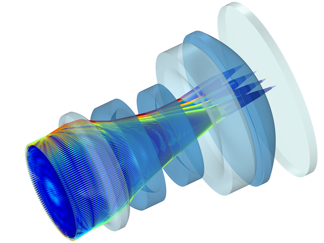
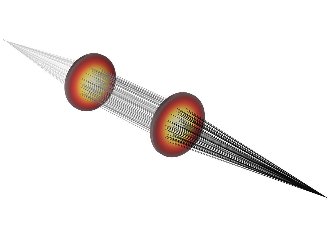
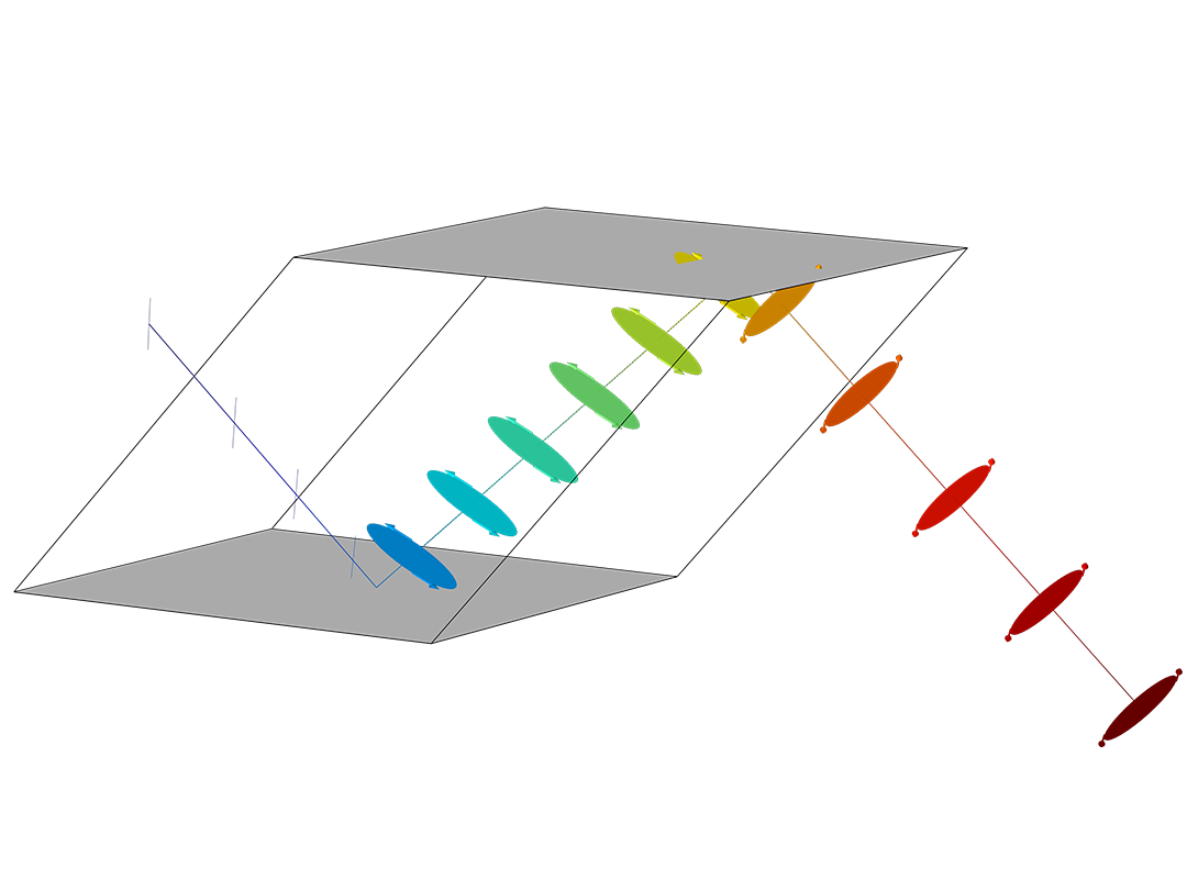
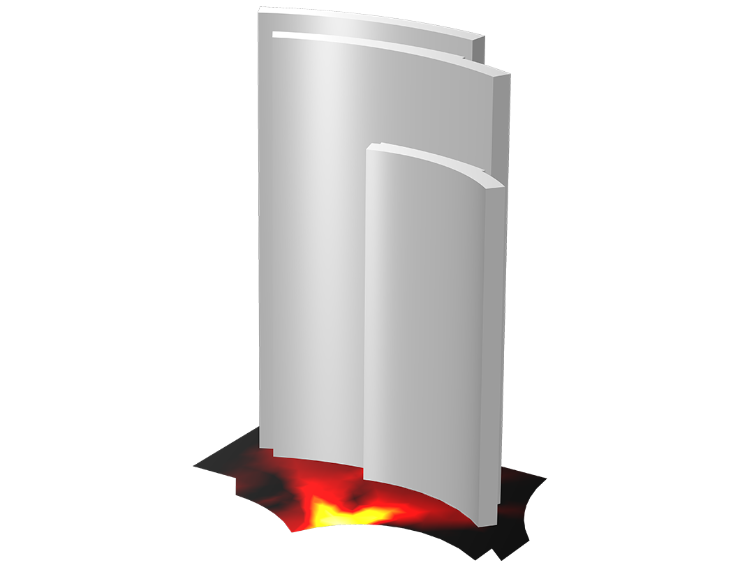
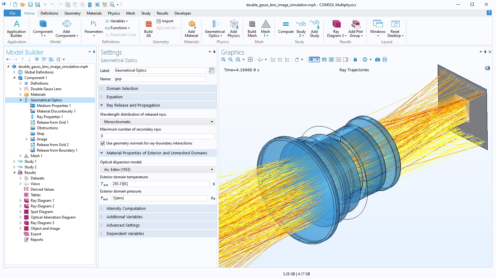
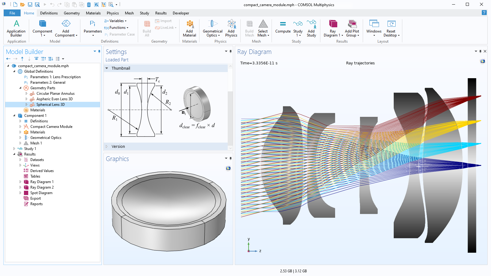
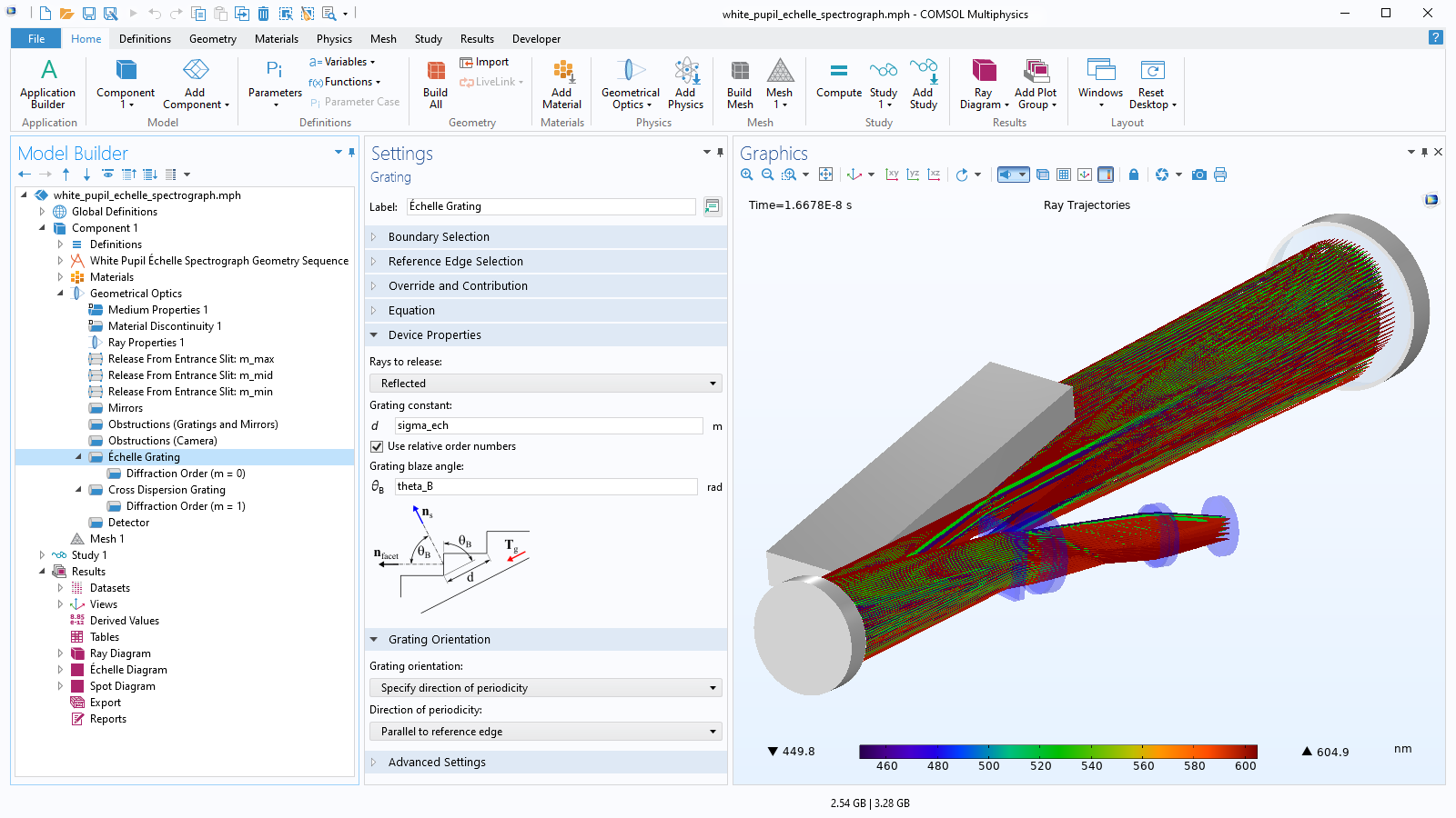
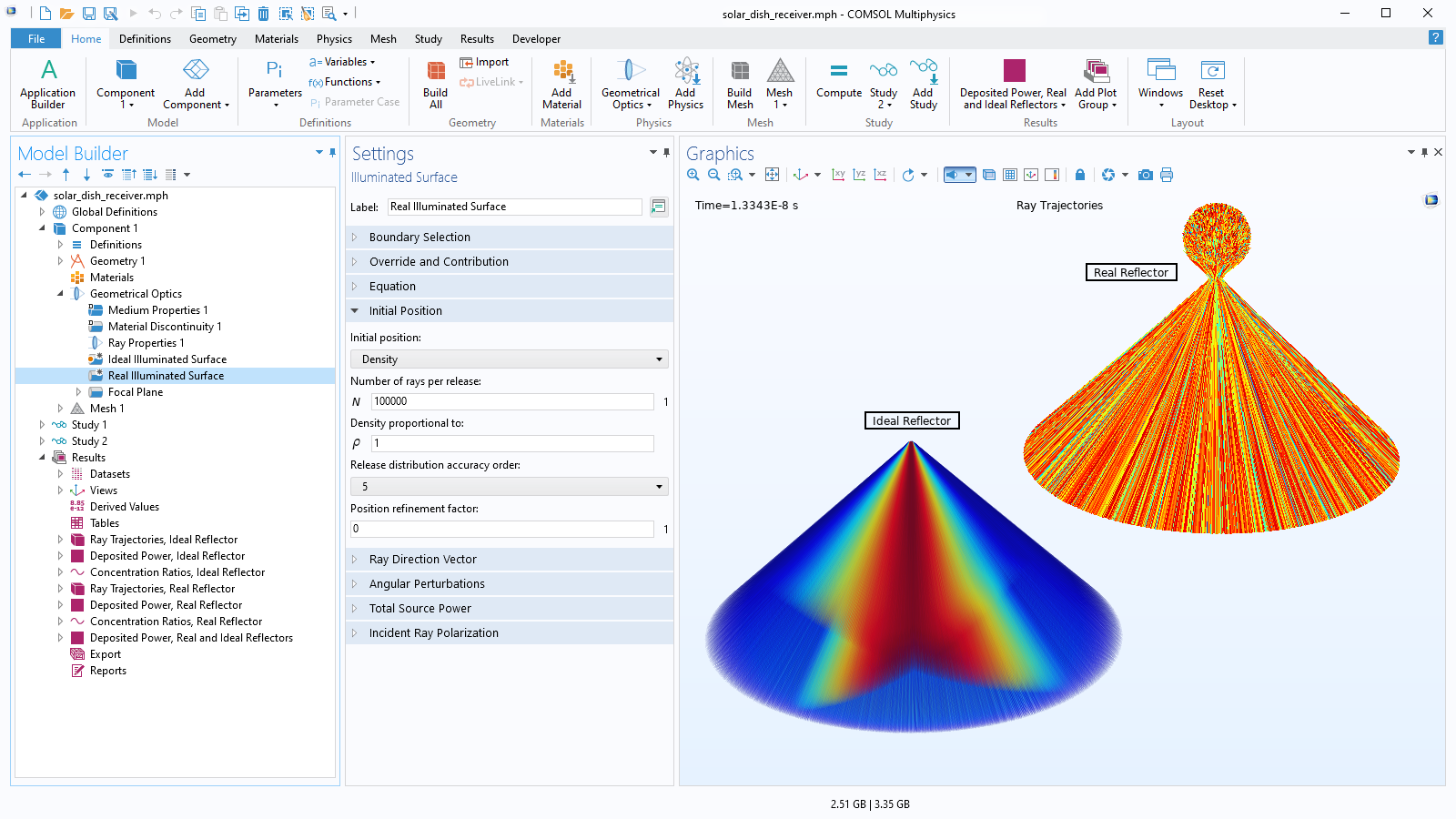
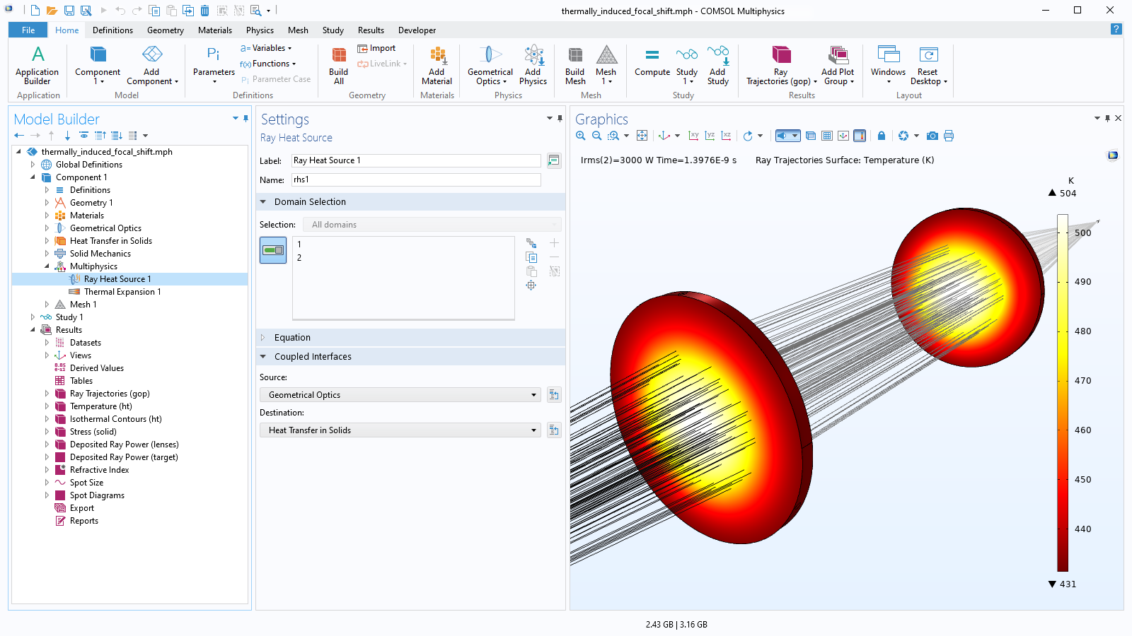
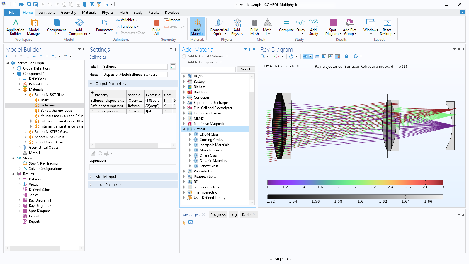
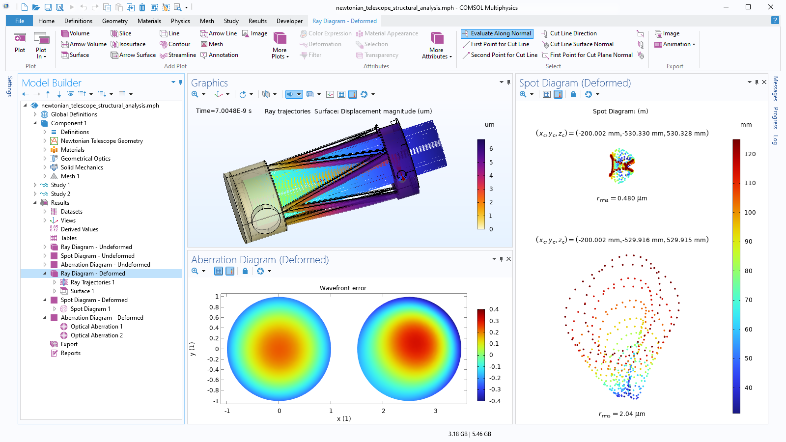
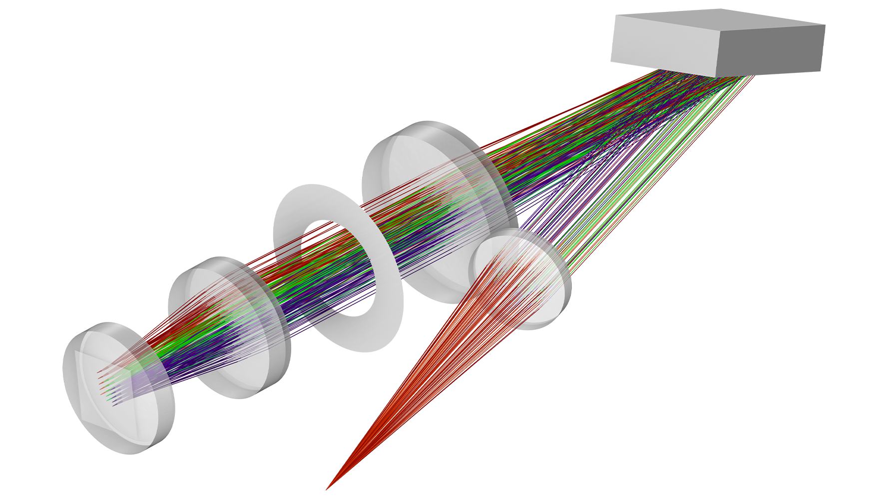
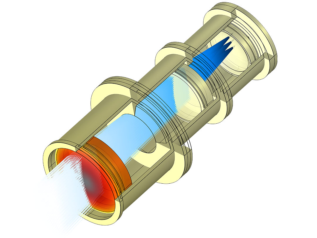
Optical systems can be extremely sensitive to changes in their environment, including high altitudes, space, underwater, and in laser and nuclear facilities. Such optical systems are subjected to structural loads and extreme temperatures. The most accurate way to fully capture these environmental effects is through numerical simulation via a STOP analysis. With the COMSOL Multiphysics® software, you can combine structural, thermal, and optical effects in a single model, so that rays are traced in the thermal-stress-induced deformed geometry while the built-in material models account for temperature-dependence of the refractive index.

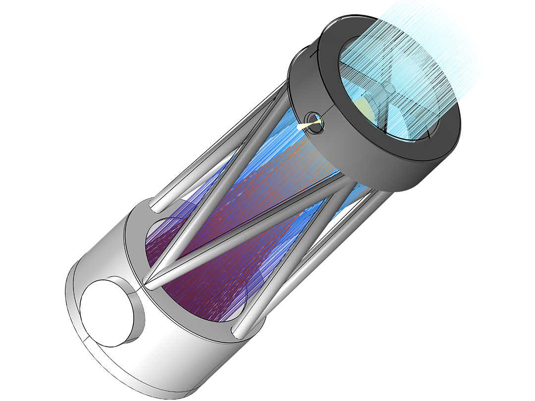
You can also combine the Ray Optics Module with other add-on modules that offer expanded structural and thermal modeling capability — for example, to account for thermal radiation, conjugate heat transfer, hyperelastic materials, and piezoelectricity.

What You Can Model with the Ray Optics Module

Perform optical ray-tracing analyses with the COMSOL® software.

A closeup view of a double Gauss lens model showing the ray trajectories and d-line refractive index.

Lenses

Analyze monochromatic aberrations of an optical system.

A closeup view of a compact camera model showing the ray trajectories.

Cameras

Design camera modules with several aspheric surfaces.

A closeup view of a bow-tie laser cavity model showing the ray trajectories.

Laser Cavities

Predict laser stability with ray-tracing capabilities.

A closeup view of a laser focusing system with ray trajectories.

Laser Focusing Systems

Trace rays through high-power laser-focusing systems.

A closeup view of a Fresnel rhomb model showing the ray propagation.

Prisms and Coatings

Manipulate the polarization of light using a built-in Stokes–Mueller formalism.

A closeup view of a Newtonian telescope model showing the deformation and ray trajectories.

Telescopes

Analyze rays of light through various telescope systems.

A closeup view of a hotel model showing the caustic surfaces at the ground.

Solar Radiation

Analyze reflected rays and solar dish concentrator/receiver systems.

A closeup view of a monochromator model showing the ray diagram.

Spectrometers and Monochromators

Separate polychromatic light using gratings or dispersive media.

A closeup view of an interferometer model with propagating rays.

Interferometers

Model ray interactions with translating and rotating surfaces.

A closeup view of a microlithography lens model showing the propagating rays.

UV Lithography

Focus ultraviolet rays to a submicron spot on a silicon substrate.

Features and Functionality in the Ray Optics Module

The Ray Optics Module uses a ray-tracing approach for modeling light propagation and electromagnetic radiation.

A closeup view of the Model Builder with the Geometrical Optics node highlighted and a double Gauss lens in the Graphics window.

Geometrical Optics

Geometrical optics can be used to model electromagnetic wave propagation in optically large structures. The Geometrical Optics interface includes built-in handling of ray intensity and polarization. The intensity calculation uses a form of Stokes–Mueller calculus that makes it easy to keep track of fully polarized, unpolarized, and partially polarized rays.

A flexible ray-tracing algorithm allows the rays to propagate through both homogeneous and graded-index (GRIN) media. They can also be monochromatic or polychromatic, where you can specify a distribution of wavelengths or enter a set of discrete values.

A closeup view of the Model Builder with the Loaded Part node highlighted and the corresponding Settings window.

Lens and Mirror Geometries

The Ray Optics Module includes a library of essential geometry parts, such as mirrors, lenses, prisms, and aperture stops. Each of these parts is fully parameterized, and many of them include variants with different combinations of input parameters so they can be conveniently modified to fit an optical design.

For example, you can insert a spherical or conic mirror into the geometry sequence; specify whether the surface is concave or convex; enter its radius of curvature; and then specify the clear diameter, full diameter, and diameter of the flat (if any). These inputs can be adjusted manually or by running a Parametric Sweep study. Additionally, the parts can be oriented with respect to previously inserted parts using built-in work planes, and the parts can automatically create named selections to easily assign boundary conditions to the correct surfaces.

A closeup view of the Model Builder with the Grating node highlighted and a spectrograph in the Graphics window.

Versatile and Intuitive Features

Rays automatically detect geometry boundaries in their path without the need to specify the order of ray–boundary interactions. When a ray reaches a surface, it can be diffusely or specularly reflected, refracted, or absorbed. You can also assign conditional boundary interactions or randomly choose between two different boundary interactions with a given probability.

At boundaries between dielectric media, each incident ray is deterministically split into reflected and refracted rays. Total internal reflection is also detected automatically. If the ray intensity is solved for, it is automatically updated for the reflected and refracted rays according to the Fresnel equations. You can also define thin dielectric layers on material discontinuities, which can be used as filters, antireflective coatings, or dielectric mirrors.

A closeup view of the Model Builder with the Illuminated Surface node highlighted and two reflector models in the Graphics window.

Ray Release Mechanisms

Rays can be initialized by entering their coordinates directly, importing the coordinates from a text file, or releasing rays from selected geometric entities. Rays can be released from any selection of domains, boundaries, edges, or points in the geometry. There are also dedicated features to produce solar radiation at a specified location on Earth's surface or to release reflected or refracted rays from an illuminated boundary.

When solving for the ray intensity, it can be initialized either by using an expression or loading a photometric data file (specifically an IES file) into the model. Additional predefined ray release features are available to model blackbody radiation and Gaussian beam propagation.

At each release position, the rays can be launched in a user-specified direction, or a number of different directions can be sampled from a spherical, hemispherical, conical, or Lambertian distribution.

A closeup view of the Model Builder with the Ray Heat Source node highlighted and two lenses in the Graphics window.

Ray Heating

The Ray Heating interface is used to model electromagnetic wave propagation in optically large systems where the rays and temperature distribution are bidirectionally, or two-way, coupled. The energy lost due to the attenuation of rays in an absorbing medium creates a heat source that is included in the temperature computation.

A closeup view of the Medium Properties node Settings window and a double Gauss lens model in the Graphics window.

Optical and Thermo-Optic Dispersion Models

The refractive index of each medium can be specified directly or derived from an optical dispersion relation. The dispersion coefficients, such as Sellmeier coefficients, can be loaded from a material database or entered directly into a user-defined material. The refractive index can be complex, wherein the real part determines the speed of light in the medium, while the imaginary part causes ray attenuation or gain.

Thermo-optic dispersion coefficients are also available to adjust the refractive index based on temperature. There is also a temperature-dependent Sellmeier dispersion model that combines the temperature and wavelength dependence into a single set of Sellmeier coefficients, which is especially useful for cryogenic materials.

A closeup view of the Model Builder with the Material node highlighted and a Petzval lens model in the Graphics window.

Optical Material Library

The Optical material library includes data for glasses from SCHOTT AG, CDGM Glass Company Ltd., Ohara Corporation, and Corning Inc., along with assorted gases, metals, and polymers. For most of these optical glasses, the refractive index is given as a function of wavelength via a set of optical dispersion coefficients.

In addition to the refractive index, many of the optical glasses in the Optical material library also provide structural and thermal properties such as density, Young's modulus, Poisson's ratio, coefficient of linear thermal expansion, thermal conductivity, and specific heat capacity. The inclusion of these structural and thermal properties further facilitates coupled STOP analysis. The internal transmittance of the glass is also tabulated as a function of wavelength, so attenuation of light in the medium can also be predicted.

A closeup view of a Spot Diagram and Aberration Diagram in two Graphics windows.

Visualization of Optical Performance

With the COMSOL Multiphysics® postprocessing tools, you have the ability to create both visually pleasing and informative simulation results. You can plot rays as lines, tubes, points, and vectors in 2D or 3D, and color the rays by an arbitrary expression that can vary between different rays and even along each ray's path. When solving for ray intensity, you can also plot polarization ellipses along the rays.

The COMSOL Multiphysics® software also provides the flexibility to show more than just ray paths, with other dedicated plots to view interference fringes and to decompose optical path difference into individual monochromatic aberration terms. You can also plot the intersection points of rays with a plane, sphere, hemisphere, or a more specialized surface.

Vdara is a registered trademark of CityCenter Land, LLC.

Every business and every simulation need is different.

In order to fully evaluate whether or not the COMSOL Multiphysics® software will meet your requirements, you need to contact us. By talking to one of our sales representatives, you will get personalized recommendations and fully documented examples to help you get the most out of your evaluation and guide you to choose the best license option to suit your needs.

Just click on the "Contact COMSOL" button, fill in your contact details and any specific comments or questions, and submit. You will receive a response from a sales representative within one business day.

Next Step

Request a Software Demonstration