MEMS Module

Analyze Microelectromechanical Systems

Microelectromechanical systems (MEMS) devices utilize electromagnetic–structure, piezoelectric, thermal–structure, and other multiphysics interactions. Understanding the interactions between various physics is crucial to successful MEMS designs, making the MEMS Module, an add-on to the COMSOL Multiphysics® software, ideally suited for analyzing MEMS devices.

Forces induced by thermal, electrostatic, and piezoelectric effects scale favorably as device dimensions are reduced. In other words, on the microscale, actuation is efficient enough to enable a range of applications that are not available on the macroscale.

Contact COMSOL
A comb-drive tuning fork gyroscope model showing the displacement magnitude in the Prism color table.

Simulate MEMS Devices and a Variety of Multiphysics Interactions

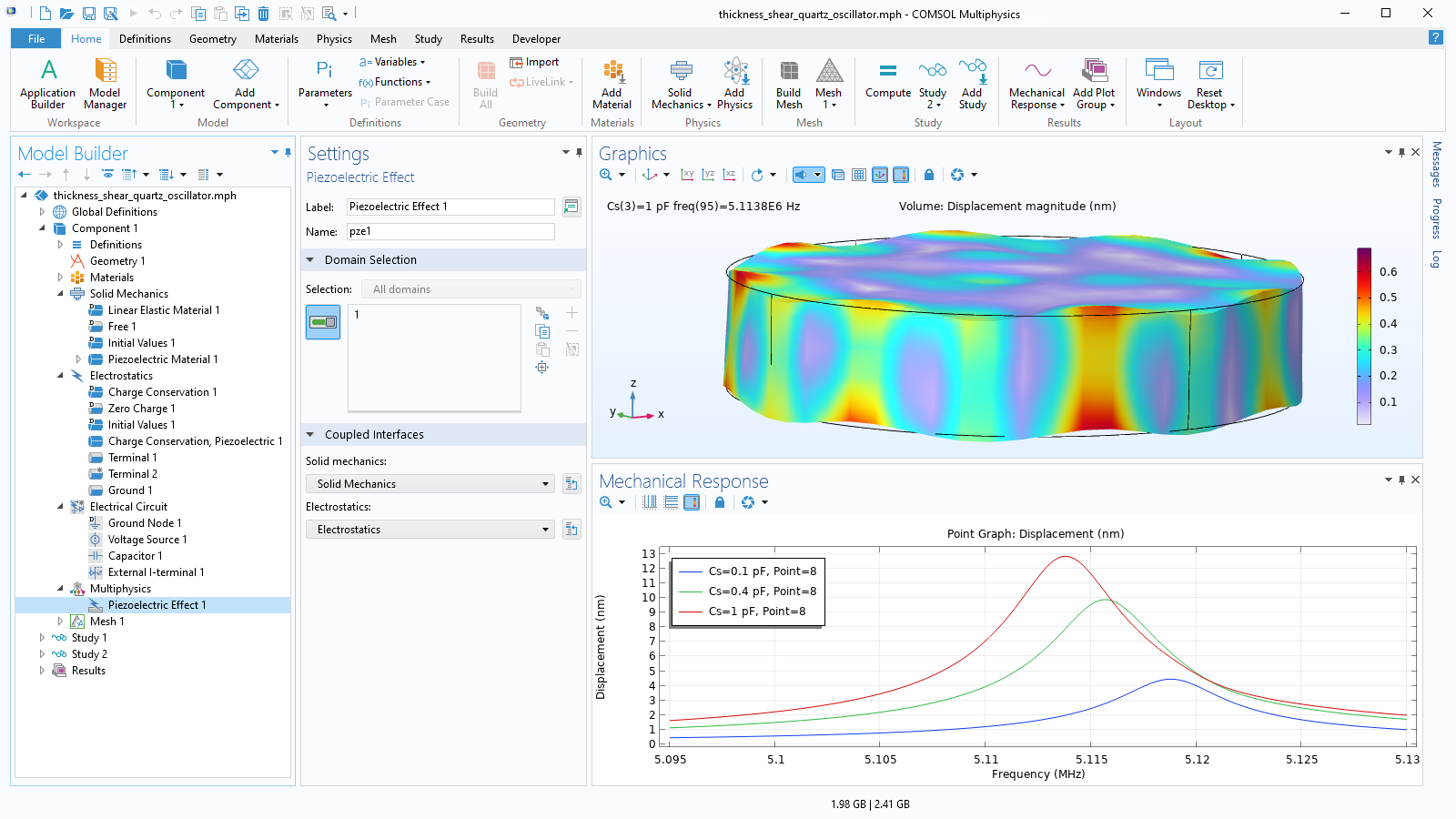
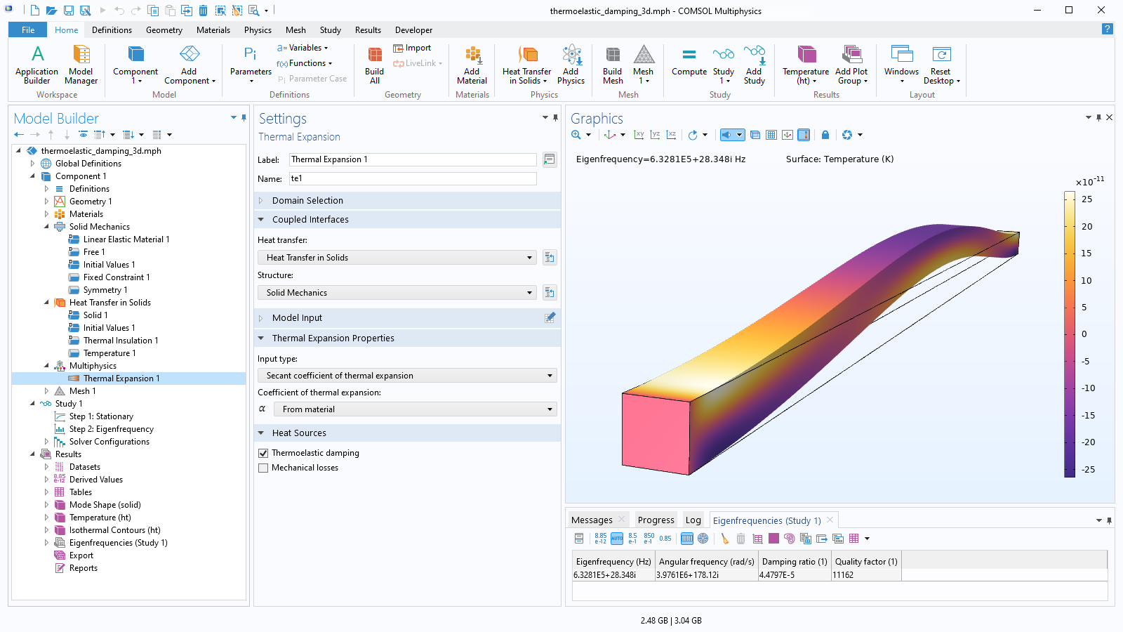
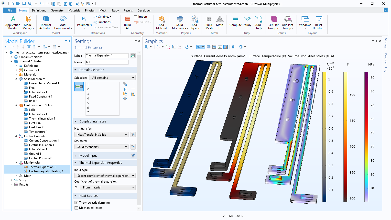
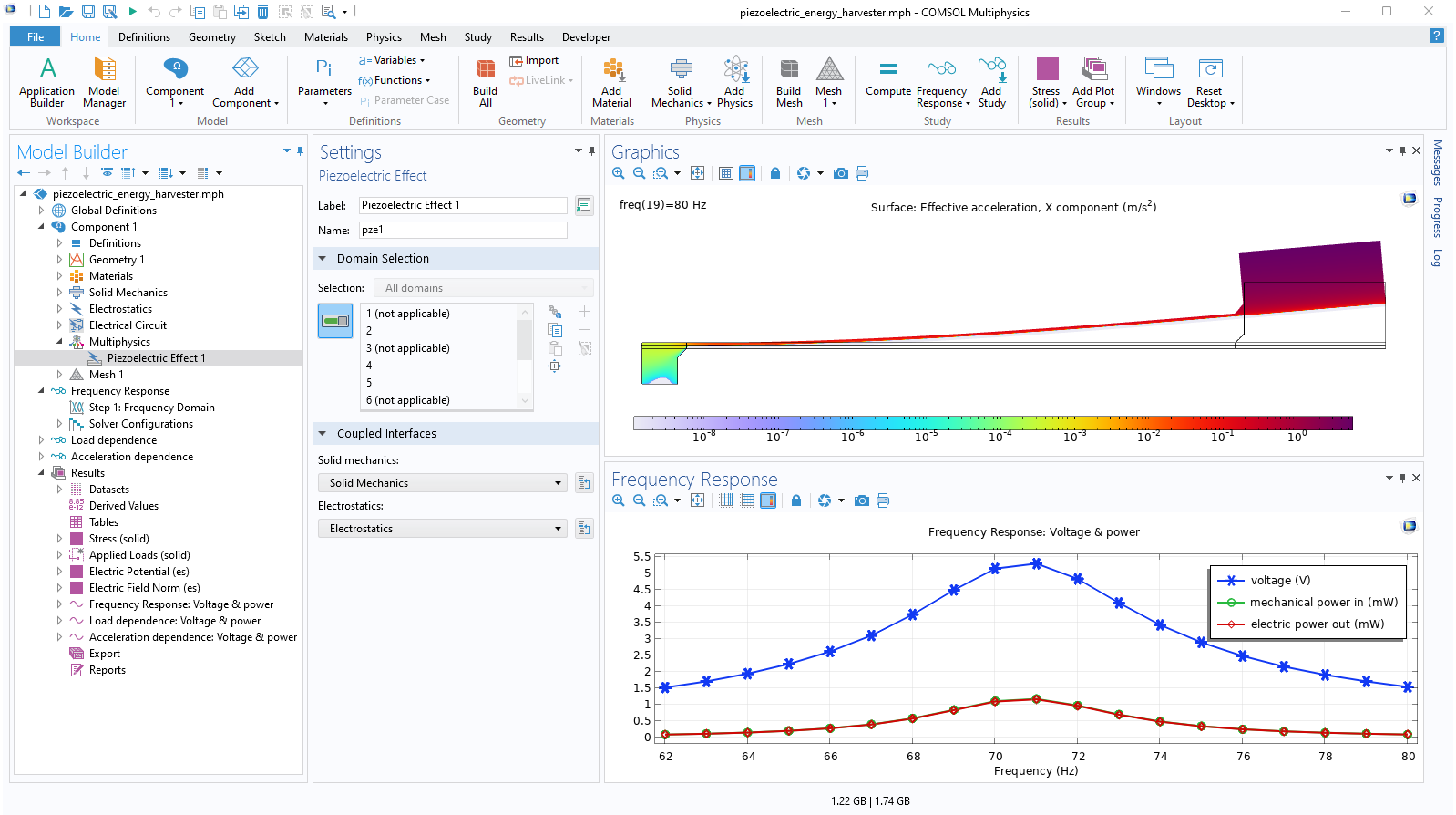
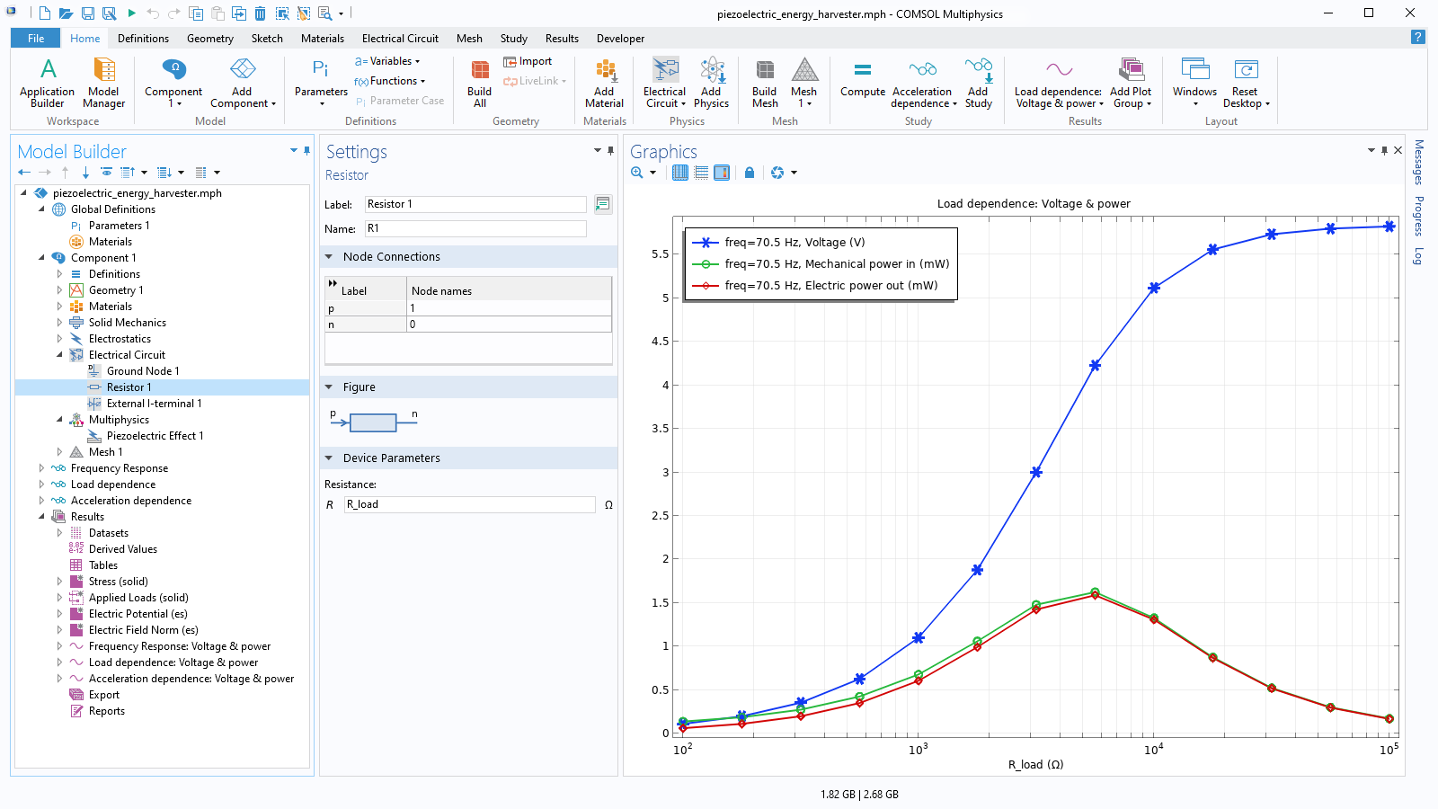
The MEMS Module is used for simulating quartz oscillators as well as many other types of piezoelectric devices. Piezoelectric simulations can include prestress as well as nonlinear effects. With the MEMS Module, you can also model the effects of thermal expansion in actuators and sensors.

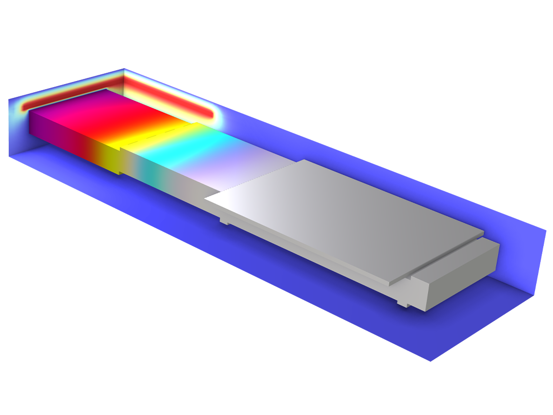
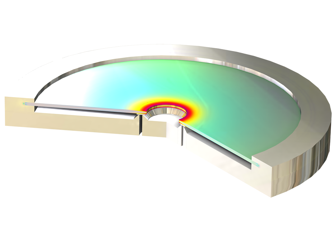
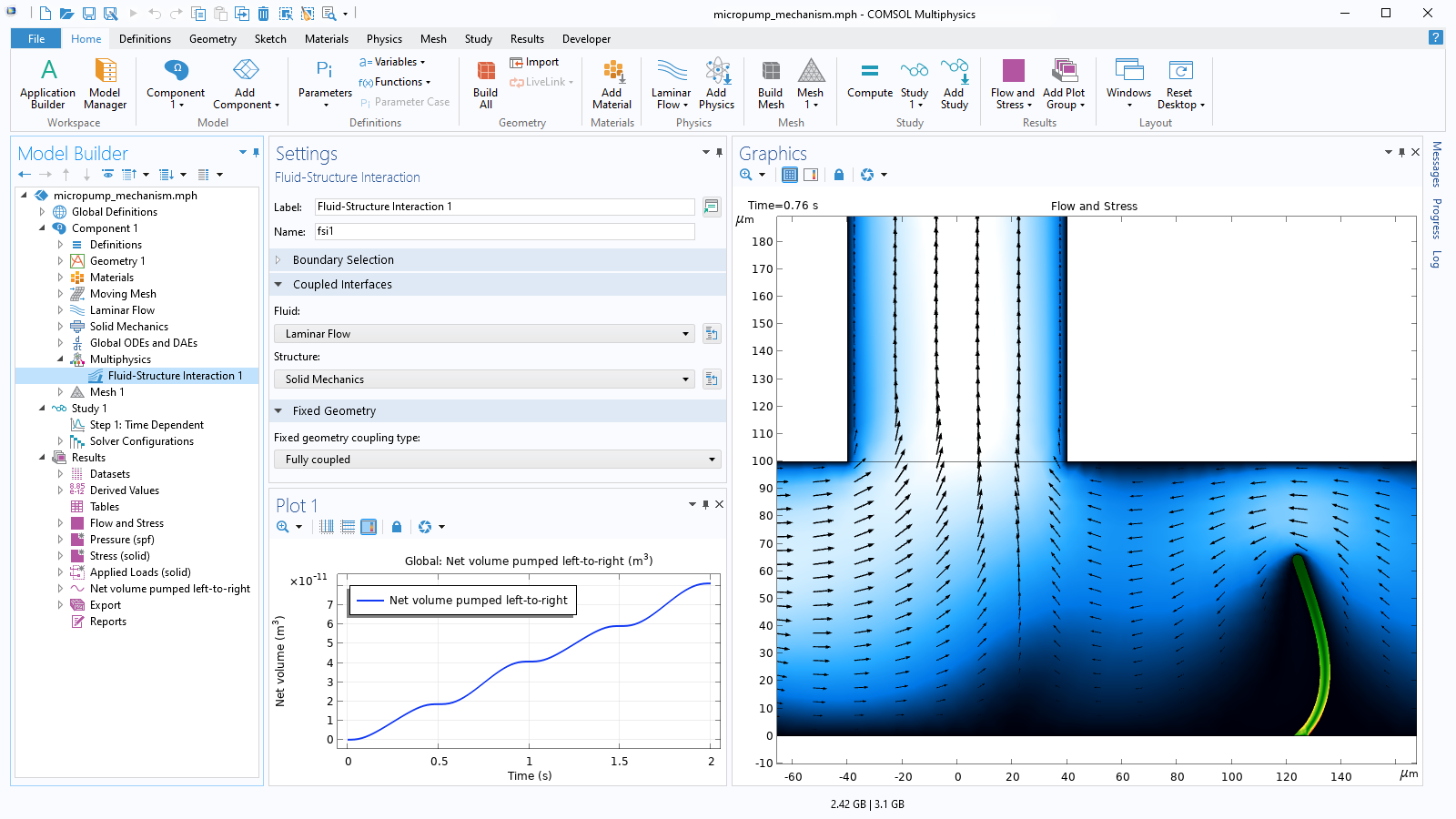
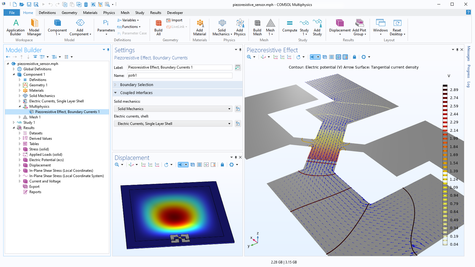
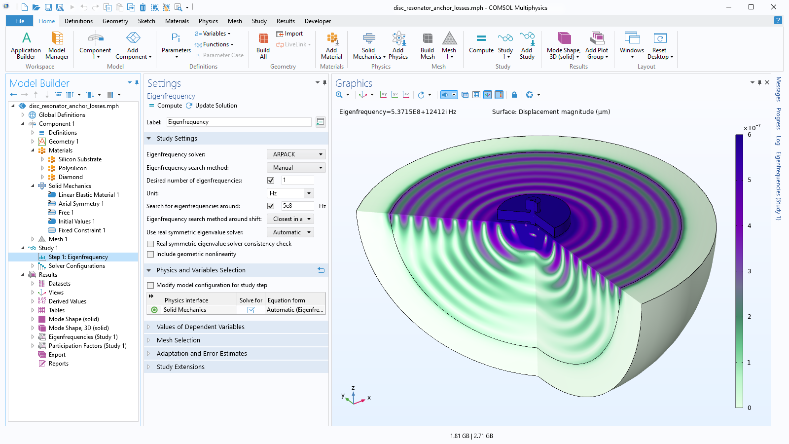
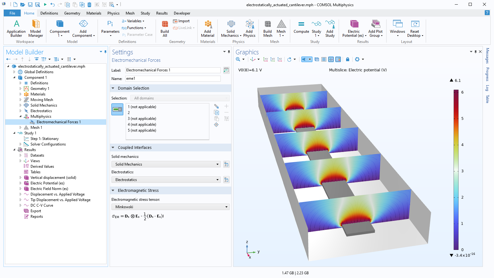
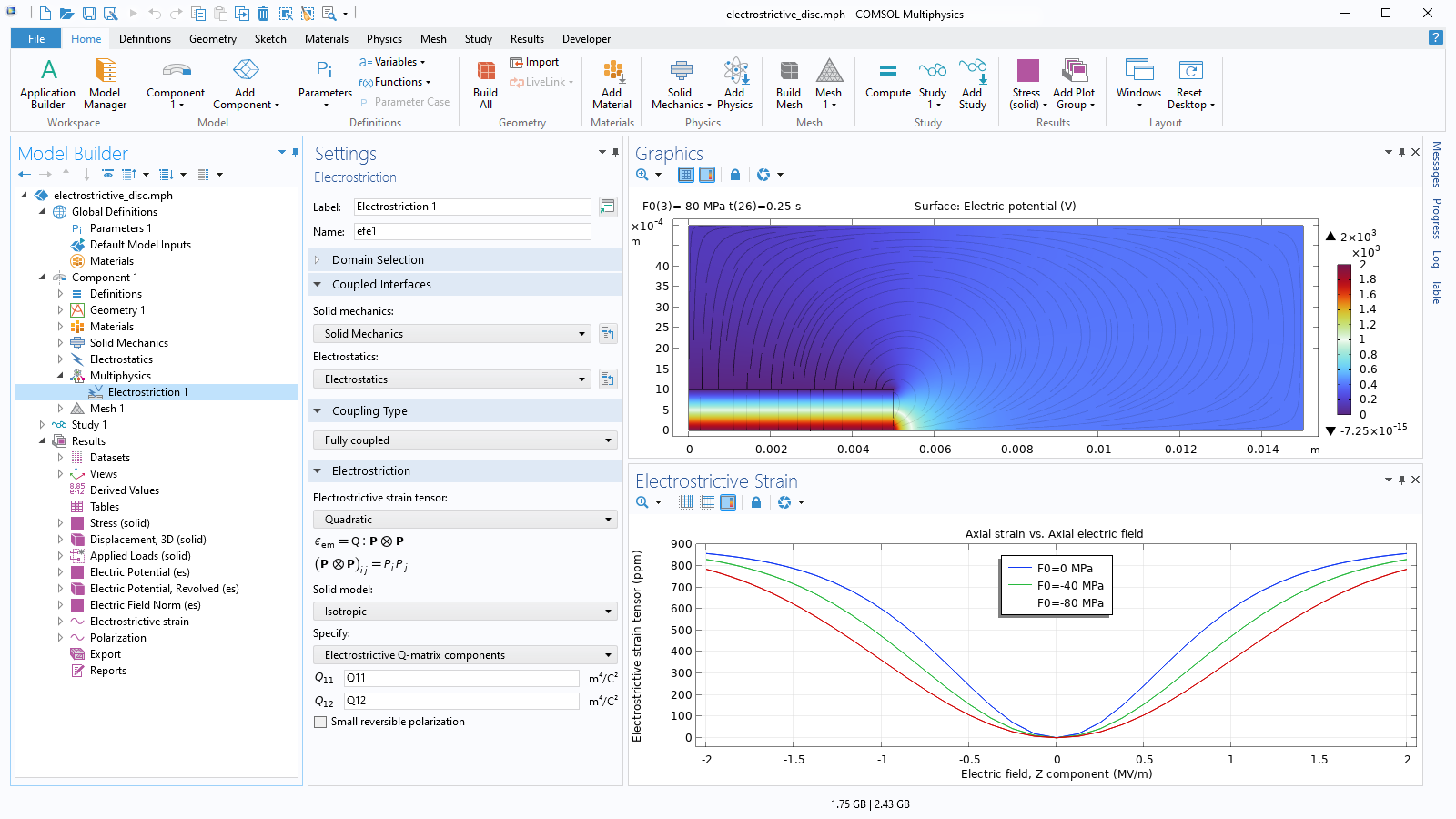
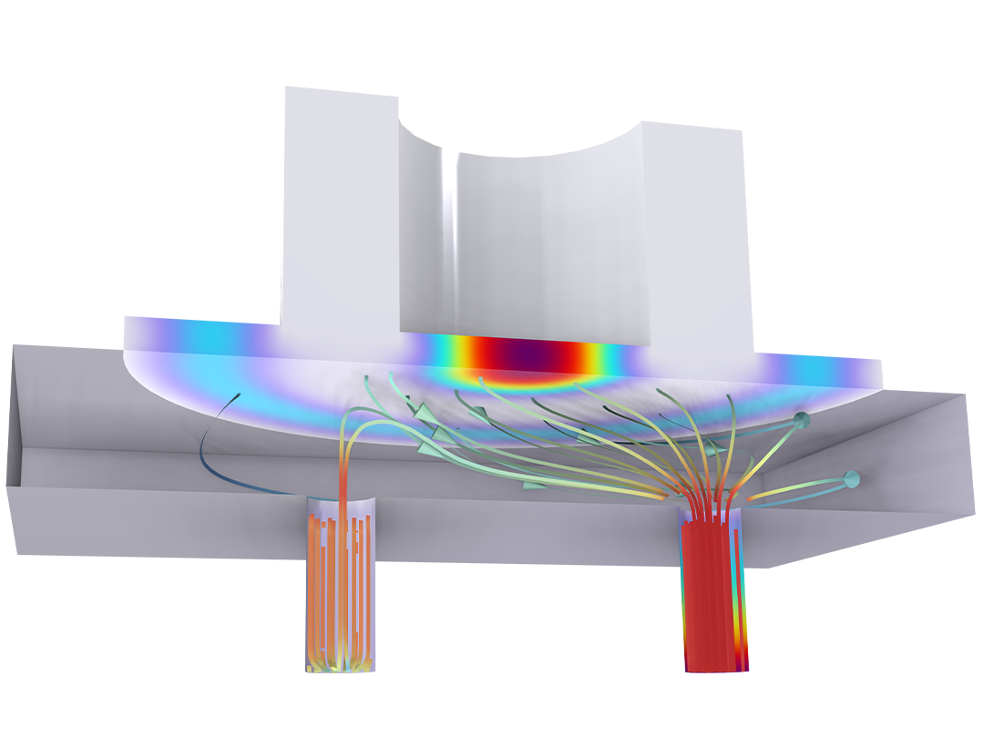
In addition to modeling common multiphysics phenomena, the MEMS Module is capable of modeling a number of intricate multiphysics interactions that are important for accurate simulation of MEMS devices. This includes hygroscopic swelling, thermoelastic and squeeze-film damping, bidirectional fluid–structure interaction (FSI), and piezoresistive, electrostrictive, and ferroelectroelastic effects (including hysteresis).

The MEMS Module can be used with other COMSOL Multiphysics® add-on modules as well. For instance, when it is combined with the AC/DC Module, you can analyze magnetostrictive devices. Working in combination with the Structural Mechanics Module enables shell modeling in MEMS devices, and adding the Microfluidics Module will provide you with additional tools for analyzing biomedical MEMS devices with an emphasis on fluid flow.

What You Can Model with the MEMS Module

Analyze a variety of MEMS devices subject to interactions between multiple physical phenomena.

A close-up view of an actuator model showing the electrothermal results.

Actuators

Simulate a wide range of actuators, including electrothermal, electrostatic, and piezoelectric actuators.

A close-up view of a pressure sensor model showing the stress.

Sensors

Predict the behavior of capacitive, piezoelectric, and piezoresistive sensors.

A close-up view of a gyroscope model showing the displacement magnitude.

Gyroscopes and Accelerometers

Analyze the electrostatic–mechanical or piezoelectric performance of gyroscope and accelerometer designs.

A close-up view of two tuning fork models.

Piezoelectric Devices

Model piezoelectric devices such as energy harvesters, transducers, actuators, and gyroscopes.

A close-up view of an oscillator model showing the mechanical response.

Quartz Oscillators

Compute the frequency response of piezoelectric crystal oscillators with arbitrary cuts and include thermal dissipation.

A close-up view of a biased resonator model showing the stress.

Electrostatically Actuated Resonators

Compute the resonant frequencies, pull-in voltage, Q factor, and the effects of different damping modes of MEMS resonators.

A close-up view of a piezoelectric valve showing the stress.

Fluidic Devices

Explore designs of micropumps, microvalves, and microfluidic sensors.

A 2D plot of a dispersion diagram.

Bulk Acoustic Wave (BAW) Resonators

Compute the frequency response and dispersion diagrams of BAW devices.

Run a Variety of Structural Analyses

The MEMS Module inherits the solid mechanics capabilities of the Structural Mechanics Module, with options for modeling solid mechanics in 3D, 2D, and 2D axial symmetry. Analyze virtually any phenomenon related to mechanics on the microscale, including contact, friction, centrifugal, Coriolis, and Euler forces. To model nonlinear materials, including hyperelastic materials, you can combine the MEMS Module with the Nonlinear Structural Materials Module.

Solid Mechanics Analyses in the MEMS Module

  • Static
  • Eigenfrequency
    • Undamped
    • Damped
    • Prestressed
  • Transient
    • Direct or mode superposition
  • Frequency response
    • Direct or mode superposition
    • Prestressed
  • Geometric nonlinearity and large deformations
  • Mechanical contact
  • Buckling
  • Response spectrum
  • Random vibration
  • Component mode synthesis

Generalized Analyses in the MEMS Module

A 1D plot of a parametric analysis with the displacement on the y-axis and force direction on the x-axis.
Parametric Analysis

Compute a model with multiple input parameters to compare results.

A close-up view of a Tesla microvalve model showing the flow field.
Optimization

Optimize geometric dimensions, shape, topology, and other quantities with the Optimization Module.

Features and Functionality in the MEMS Module

The MEMS Module contains specialized features and functionality for modeling MEMS devices.

A close-up view of the Model Builder with the Piezoelectric Effect node highlighted and an oscillator model in the Graphics window.

Built-In User Interfaces and Results

The MEMS Module provides built-in user interfaces that are tailored to the type of device and multiphysics interaction you are analyzing. These interfaces define sets of domain equations, boundary conditions, initial conditions, predefined meshes, and predefined studies with solver settings as well as predefined plots and derived values. All of these features can be accessed within the COMSOL Multiphysics® environment.

Values for the electric field, stress, strain, quality factors, damping, resonant frequencies, dissipation, and scattering parameter (S-parameter), as well as values for capacitance, admittance, and impedance matrices, can be calculated and exported to the Touchstone file format. You can plot or evaluate any mathematical expression in terms of the computed quantities.

A close-up view of the Model Builder with the Electrostatics, Boundary Elements node highlighted and a tunable capacitor model in the Graphics window.

Electrostatics

You can analyze the capacitive effects in MEMS devices with electrostatics computations where the fields are determined by the electric potential and charge distribution. Both the finite element method (FEM) and boundary element method (BEM) are available for solving the electric potential and can be combined for a hybrid boundary-element–finite-element method (BEM–FEM). Based on the computed potential field, a number of quantities can be calculated, such as the capacitance matrices, electric fields, charge density, and electrostatic energy.

The electrostatics functionality can be extended with built-in options for multiphysics effects like piezoelectricity, electrostriction, and ferroelectricity. Debye dispersion and dielectric loss material models are available for both frequency-domain and time-dependent analysis.

A close-up view of the Model Builder with the Fluid-Structure Interaction node highlighted and a micropump model in the Graphics window.

Fluid–Structure Interaction (FSI)

The Fluid-Structure Interaction (FSI) multiphysics interface of the MEMS Module combines fluid flow with solid mechanics to capture the bidirectional interactions between fluids and solid structures. The flow can be either laminar or turbulent. For including specific microfluidic phenomena, you can combine the MEMS Module with the Microfluidics Module. Turbulent flow requires the CFD Module or Heat Transfer Module. The CFD Module also allows two-phase and three-phase flow to be coupled with solid mechanics.

A close-up view of the Model Builder with the Piezoresistive Effect, Boundary Currents node highlighted and a piezoresistive sensor model in the Graphics window.

Piezoresistivity

The piezoresistive effect refers to the change in a material’s conductivity in response to an applied stress. The ease of integration of small piezoresistors with standard semiconductor processes, along with the reasonably linear response of the sensor, has made this technology particularly important in the pressure sensor industry. For modeling piezoresistive sensors, the MEMS Module provides several dedicated interfaces for piezoresistivity in solids or shells. When combining the MEMS Module with the Structural Mechanics Module, a piezoresistivity user interface for thin shells is available.

A close-up view of the Model Builder with the Thermal Expansion node highlighted and a resonator model in the Graphics window.

Thermomechanical Couplings

The Thermoelasticity interface combines the Solid Mechanics and Heat Transfer in Solids interfaces, which includes coupling terms for thermoelastic damping. Thermoelastic damping is particularly important in smaller MEMS structures, in which regions of compression and expansion are in close proximity. The cyclic deformation of resonators creates local temperature variations and thermal expansion of the material, which appears as damping. The thermoelastic coupling terms result in the material being cooled when under tension and heated when under compression. The resulting irreversible heat transfer between warm and cool regions of the solid produces mechanical losses that may be important at the microscopic level.

A close-up view of the Model Builder with the Eigenfrequency node highlighted and resonator model in the Graphics window.

Damping in MEMS Resonators

A number of different damping phenomena can be modeled using the MEMS Module, including squeeze-film damping; isotropic and anisotropic loss-factors for dielectric, elastic, and piezoelectric materials; and thermoelastic damping. For computing anchor damping, perfectly matched layers (PMLs) provide state-of-the-art absorption of outgoing elastic waves for both elastic and piezoelectric solids. You can perform a fully coupled eigenfrequency, frequency-response, or transient analysis.

By combining the MEMS Module with the Acoustics Module, you can include the effects of acoustic damping from a surrounding fluid, including pressure acoustic and thermoviscous acoustic damping.

A close-up view of the Model Builder with the Terminal node highlighted and a MEMS resonator in the Graphics window.

Prestressed and Biased Devices

The MEMS Module can be used to study devices that are prestressed with mechanical and thermal loads. The built-in harmonic perturbation analysis allows for computing the frequency response as well as the eigenfrequencies and eigenmodes of such models.

In a similar way, electrostatically biased MEMS resonators, including micromechanical filters, can be analyzed. For instance, since these devices are biased by a DC voltage and driven by an alternating current, you can analyze how damping and biasing effects cause the resonance frequencies to shift.

A close-up view of the Model Builder with the Thermal Expansion and Electromagnetic Heating nodes highlighted and three actuator results in the Graphics window.

Joule Heating and Thermal Stress

You can easily combine thermal, electric, and structural multiphysics effects. Predefined multiphysics couplings for Joule heating and thermal expansion enable you to model the conduction of electric current in a structure, the subsequent electric heating caused by the ohmic losses, and the thermal stresses induced by the temperature field. Typical applications include thermal actuators and fuses. All material properties are allowed to be nonlinear and temperature dependent. Modeling of mechanical contact can be extended to include contact resistance for both heat and electric currents. Thin conducting layers can be modeled using specialized tools for layered shells.

A close-up view of the Model Builder with the Piezoelectric Effect node highlighted and an energy harvester model in the Graphics windows.

Piezoelectricity

Uniquely advanced piezoelectric modeling tools allow for static, frequency-domain, coupled eigenfrequency, and time-domain simulations. Designs are allowed to have materials combined in any imaginable configuration and can easily include coupled piezoelectric, metallic, dielectric, and fluid parts.

Both the direct and inverse piezoelectric effects can be modeled, and the piezoelectric coupling can be formulated using the strain-charge or stress-charge forms. The MEMS Module includes a library of common piezoelectric material properties, including lead zirconate titanate (PZT) and quartz properties. Many piezoelectric materials exhibit nonlinear ferroelectroelastic behavior at large applied electric fields. You can model thin-layered dielectric and piezoelectric structures with shells, which you can access by combining the MEMS Module and Composite Materials Module.

Damping in piezoelectric devices can be represented with loss factors for the piezoelectric as well as the elastic and dielectric parts. Dielectric heating can be computed and coupled with heat transfer analysis to investigate the effects of dispersion.

When analyzing piezoelectric behavior using the Piezoelectricity interface, you can get results for the electric potential and electric field, displacement, strain, stress, capacitance, losses, admittance, impedance, and S-parameters.

A close-up view of the Model Builder with the Frequency Domain node highlighted and a 1D plot in the Graphics window.

Wave Dynamics in Elastic and Piezoelectric Materials

Vibrations and propagation of elastic and piezoelectric waves can be modeled in the frequency domain as well as in the time domain. This enables analysis of, for example, acoustic transducers and resonators, including bulk acoustic wave (BAW) devices.

For time-domain simulations, you can choose between implicit and explicit methods. In all cases, different material types can be combined in the same model, including functionally graded materials.

The frequency-domain and implicit time-domain simulations are based on the finite element method, whereas the explicit time-domain simulations are based on the discontinuous Galerkin (dG or dG-FEM) method. The dG-FEM method uses a time-explicit solver to ensure a computationally efficient hybrid method that can solve very large models with many millions of degrees of freedom (DOFs). This method shows excellent parallel computing performance, including when you run it on clusters.

For modeling waves leaving the computational domain, a variety of boundary conditions and absorbing layers are available, including nonreflecting boundary conditions, sponge layers, perfectly matched layers (PMLs), and elastic port boundary conditions.

A close-up view of the Model Builder with the Electromechanical Forces node highlighted and a cantilever model in the Graphics window.

Electromagnetic–Structure Interaction

The Electromechanics multiphysics interface combines solid mechanics and electrostatics with a moving mesh to help you model the deformation of electrostatically actuated structures, such as inertial sensors. The interface is also compatible with ferroelectroelastic and electrostrictive materials and has options for both FEM and BEM. A similar multiphysics interface for magnetomechanics is available when the MEMS Module is combined with the AC/DC Module.

A close-up view of the Model Builder with the Electrostriction node highlighted and two Graphics windows.

Electrostrictive and Ferroelectroelastic Materials

Electrostriction is a form of electromechanical interaction where an electric field applied to an electrostrictive material generates a deformation of the material (direct effect), and a stress applied to the material changes its polarization (inverse effect). To model this phenomenon, you can use the Electrostriction interface, which includes a multiphysics coupling between the Solid Mechanics and Electrostatics interfaces.

The Ferroelectroelasticity interface can be used for modeling the coupling of Solid Mechanics and Electrostatics. This enables you to model nonlinear electromechanical interactions in ferroelectric and piezoelectric materials. Electric polarization in such materials, including possible hysteresis and saturation effects, depends nonlinearly on the applied electric field. In addition, the polarization and mechanical deformations in such materials can be strongly coupled.

A close-up view of the Model Builder with the Resistor node highlighted and a 1D plot in the Graphics window.

Electrical Circuits

The MEMS Module allows you to combine 2D and 3D models with SPICE circuits. In the combined simulation, parts of the model will have circuit representation. This can be used to evaluate the effect of a series capacitor on a quartz crystal oscillator, for example.

For any model or combination of models, you can use the Electrical Circuit interface to solve for the voltages, currents, and charges associated with the circuit elements. Circuit models can contain passive elements like resistors, capacitors, and inductors as well as active elements such as diodes and transistors. You can export and import circuit topologies in the SPICE netlist format.

Create and Import MEMS Designs

You can choose to create your geometric design within COMSOL Multiphysics® using the built-in CAD tools or by importing files created with another software program.

To make it easy for you to perform analyses based on mechanical CAD models, COMSOL offers the CAD Import Module, Design Module, and LiveLink™ products for several leading CAD systems as part of its product suite.

For importing electronic layout files, including files in the GDSII format, you can use the ECAD Import Module. You can also freely combine ECAD and mechanical CAD models.

Every business and every simulation need is different.

In order to fully evaluate whether or not the COMSOL Multiphysics® software will meet your requirements, you need to contact us. By talking to one of our sales representatives, you will get personalized recommendations and fully documented examples to help you get the most out of your evaluation and guide you to choose the best license option to suit your needs.

Just click on the "Contact COMSOL" button, fill in your contact details and any specific comments or questions, and submit. You will receive a response from a sales representative within one business day.

Next Step

Request a Software Demonstration