

Whenever we are solving a thermal problem where radiation is significant, we need to know the emissivities of all of our surfaces. Emissivity is a measure of the ability of a surface to emit energy by radiation, and it can depend strongly upon the wavelength of the radiation. This is very relevant for thermal problems where the temperature variation is large or when there is exposure to a high-temperature source of radiation such as the sun. In this post on thermal modeling, we will look at how to include wavelength-dependent surface emissivities in a problem that is of importance to everybody: Having a relaxing day at the beach!
Staying Cool at the Beach: A Thermal Modeling Scenario
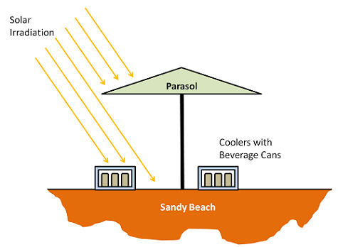
The problem we will look at is of two styrofoam coolers containing beverage cans that are initially at 1°C. The coolers are on a sandy beach, and a parasol overhead will provide partial shade during the course of the day. We want to find out how long it takes for the beverage cans to warm up. But before we do that, let’s look at some of the fundamentals.
Understanding Surface Emissivity
If we have a surface of temperature T exposed to ambient conditions at a lower temperature, T_{amb}, then the surface will radiate at many wavelengths, and the total radiative heat flux is:
where \epsilon is the wavelength-dependent emissivity, and \sigma is the Stephan-Boltzmann constant. If the emissivity is unity, then we would say that the surface is an ideal black body, but all real surfaces have an emissivity that is less than unity.
The above equation is reciprocal, that is, it holds equivalently if the surface is hotter or colder than ambient. Another way of saying this is that the emissivity equals absorptivity, where absorptivity is the measure of how much of the incident radiation is absorbed by a surface. From here on we will use these terms interchangeably.
So if we know the incident radiative flux on a surface and the surface absorptivity, then we know how much heat is being absorbed. We will assume that we are dealing with opaque materials, so all incident radiation is either absorbed or reflected, and there is no transmission of radiation through the cooler walls. Keep in mind that emissivity is not just a material property, but can also be a function of the surface treatment. A matte surface and a very smooth surface made of the same material can have different emissivities. We will also assume diffuse reflections, and neglect any directional dependence of absorptivity, a valid assumption unless we are dealing with highly polished surfaces like mirrors.
Now the interesting part of this analysis will be that the surface absorptivity (emissivity) of our coolers varies quite significantly with wavelength. This wavelength dependence is important because we have radiative heat transfer in different spectral bands.
Understanding Spectral Dependency of Radiation
An object can be considered a black body if it emits electromagnetic radiation following Planck’s Law. A good example is the sun; the solar spectral distribution follows very closely to that of a black body at 5,800 K if we are outside of the atmosphere. The earth’s atmosphere absorbs some of this energy, but at ground level the shape of the spectrum is still quite close to that of a black body. For a lot of problems of engineering interest, the peak temperatures will not get above 500 K, so let’s look at the fraction of energy emitted at each wavelength for a black body at 5,800 K and 500 K.
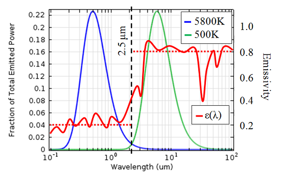
Fraction of total emitted power as a function of wavelength for a black body at different
temperatures. The wavelength-dependent emissivity of the cooler is also plotted, in the
solar band the average emissivity is 0.2, while in the ambient band an average of 0.8 is a
good approximation.
We can see that most of the radiated energy from a 5,800 K object is in the spectral band of wavelengths shorter than 2.5 microns, whereas most of the energy from the 500 K object is radiated at wavelengths longer than 2.5 microns. When we overlay the emissivity of our coolers onto this graph, we see that the wavelength-dependence of emissivity is quite important.
The engineers who designed these coolers chose a material with a low absorptivity in the solar spectral band, meaning that only a small fraction of the incident solar radiation is absorbed. On the other hand, in the long-wavelength spectral band the emissivity is higher, meaning that, since the coolers will be much less than 500 K, it is easy for heat to radiate away.
Putting It Together in COMSOL
When you are using the Heat Transfer Module, you have the option to specify wavelength-dependent emissivities. It is often sufficient to use only two spectral bands, as shown above, but you can have up to five. Although emissivities can vary strongly with wavelength, it is often sufficient to use an average value over the band, or to choose the value corresponding to the expected peak in the black body spectral distribution.
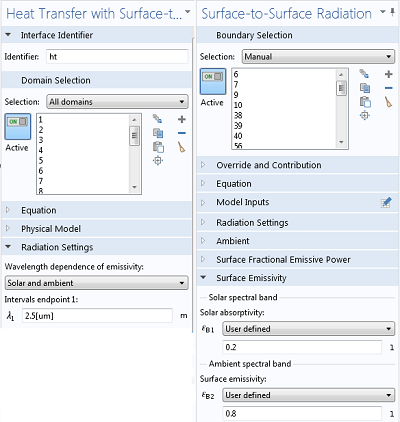
Settings for handling multiple spectral bands.
We will include an External Radiation Source feature to model the solar irradiation. This allows us to enter a latitude, longitude, and time of day, as well as a solar irradiance. COMSOL will compute the incident solar heat flux, and consider the shadowing due to the parasol.
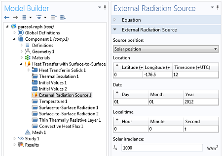
Settings for the External Radiation Source.
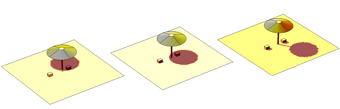
Solar irradiation at three different times of day.
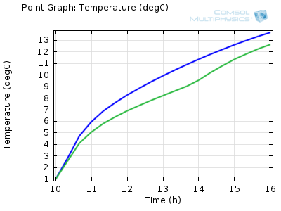
Temperature of a beverage can inside the shaded (green) and
unshaded (blue) cooler over time.
Summary and Next Steps
We can see from the results that the beverage cans in the shaded cooler will stay below 10°C for about an hour and a half longer than those placed in the direct sunlight. This means that you have more time to relax with a cold drink on the beach!
Whenever you are dealing with a thermal problem where your system is exposed to sunlight, or if you have large temperature variations in your system, you can have radiation in multiple spectral bands and will need to consider wavelength-dependent emissivity. This functionality is available in the Heat Transfer Module.
If you would like to learn how to set up this kind of model yourself, check out our Parasol model. If you are interested in using COMSOL Multiphysics for your thermal modeling needs, please contact us.

Comments (8)
William Afonso
November 6, 2017Hello,
I understand we can specify different emissivities for one to five wavelength intervals in COMSOL.
However, I would also like to specify a particular irradiance for short wavelengths and another one for long wavelengths.
Does anyone knows how to do it?
Walter Frei
November 6, 2017Hello William,
You would use the “External Radiation Source” feature for this, similar to what is shown in the above screenshot, but specify a “User defined” source power definition.
Mushtaq Al-asadi
November 20, 2017Dear Dr Walter,
I really need your help, I have a look at all the blogs posting. Please I am working in Solar air collectors or systems. Below is the brief description:
Air solar collectors are a kind of heat exchangers that transform solar energy into heat.
Typical air solar collectors consist of a case, which holds a back insulation, an absorber and a transparent cover (glass). The transparent cover reduces heat losses towards the front, meanwhile the air flows in between the absorber plate and the thermal insulation.
I have seen all your blogs and I can not get any related tutorial or blog.
the issue is, I am stuck since months in how to simulate or model the glass cover correctly in terms of the effect of absorption, emission and reflection. The thickness of glass cover is between 3-5 mm. Please, it will be very helpful if you offer any help.
shimin li
July 14, 2019Dear Mushtaq and Walter,
I am glad to find your comments above. Now I meet the same question with you. Could you share you final solution with me. Thank you very much!!!
I want to set a PE thin film on our structure, this film is transparent in solar and IR wavelength.
Radiation cooling on earth is my project, so how to modeling the atmosphere in simulation is anther big problem for simulation. (Atmosphere is a half transparent layer in 8-13um in IR wavelength range. )
Salman Ahmed
April 15, 2020Hello shimin li. I saw your comment regarding radiative cooling and thought of messaging you since I am working on the radiative cooling of solar panels. I had some questions regarding its modeling. Can we talk?
Ivar KJELBERG
February 1, 2022Hi Walter,
I’m coming back to this Blog page (almost 10 years old! but still instructive and valid ;), following your newer, and complementary page: https://www.comsol.com/blogs/modeling-emissivity-in-radiative-heat-transfer/
I would like to give some precision on your choice of choosing 2.5[um] wavelength as an emissivity limit between thermal and visible solar radiation. Your blog show many curves that are fully valid, but “theoretical”, for practical work we also need to look at the integrated values, not only the total energy (for emissivity=1 and a view factor of one) of sigma_boltzmann*T^4 but also the fractional ones up to and below this chosen wavelength limit.
As you show here above, the spectral signal height of the solar flux and the 500[K] flux is about the same at 2.5[um] so you choose this as a limit. Fully valuable for given cases, but if you take the total solar flux, at the level of the Earth, even if “sigma_const*(5777[k])^4” ~ 6.32E7[W/m^2] we live, on Earth, at some 215 times away from the emission radius of the sun, so the total energy flux reaching us is reduced to some 6.32E7[W/m^2]/(215^2) ~ 1360[W/m^2], and typically some 1-0.8[kW/m^2] reaches the Earth surface where we live, the rest being absorbed by the atmosphere.
Now, an object at 500[K] has a blackbody irradiance of some 3544 [W/m^2], far more than that from the sun.
While for Earth’s average temperature is only of some 15[degC] the total emitted energy is only some sigma_const*(273.15[K]+15[K])^4 ~ 390[W/m^2] or a half to one third of the effective sun irradiance.
Now, if we integrate the blackbody spectra (still emissivity = 1) from 2.5[um] to +INF for a source of temperature 5777[K] we get to ignore some ~46.5[W/m^2] due to the highly asymmetric Boltzmann distribution, while 0-2.5[um] wavelength covers quasi the total emissive power of a source of 300[K] and leaves out only ~11[W/m^2] for a source of temperature 500[K] (this is only really visible on log-log graphs of the blackbody emissive spectral power). Hence, at 2.5[um] cutoff wavelength we have some 46.5/390 or ~12% error on the total solar irradiance with respect to the Earth mean temperature irradiance, and a factor 4 on the integrated radiated power between the sun spectra and the 500[K] sources.
Therefore for my more human temperature cases, I usually use 5[um] as a cutoff wavelength for the sun illumination, this also corresponds to the integrated power balance for “human” temperatures, but I agree it is quite too far-fetched for a 500[K] source that fits better to a 2.5[um] limit, due to the highly non-linear T^4 relationship here.
Another argument is that 5[um] is the cutoff wavelength for the transmission of most “spacecraft windows” in fused Quartz or Sapphire so it corresponds to a natural bandpass, a mix of material transmission filter and emissivity values, since these are highly linked.
Note that for most terrestrial cases, we are considering sun light behind a float glass window, and the transmission limit is here closer to 2.5[um] so for these cases of greenhouse analysis for houses and building the 2.5[um] wavelength limit is better.
So nothing wrong with the 2.5[um] limit, but one should adapt it better to each case by quickly calculating out the total energies in play for a given case, and nothing easier to do this directly in COMSOL, as parameters or functions, and call this a first approach VV&C activity, something one should always do for all models.
Sincerely,
Ivar
Still, after soon 20 years, having great fun COMSOLing …
Walter Frei
February 1, 2022 COMSOL EmployeeThank you Ivar, for the detailed reply. I should also add that the 2.5um division chosen here is indeed a bit arbitrary. (I do believe that somewhere in the range of 2-5um is typical.) From the point of view of the software, though, we strive to make clear that these kinds of choices are fully the users’ responsibility. Depending upon if we’re above or below the atmosphere, the expected temperature range, and depending upon the materials that we are working with, we may well want to a different division.
Again, thank you for demonstrating the importance of this kind of pre-analysis calculation.
Ivar KJELBERG
February 2, 2022Hello Walter,
Exactly, default values are necessary, but should be regularly questioned (by the users), as each model case is different.
But nothing easier to set up a few Parameters and Functions in COMSOL Multiphysics® to check them out for a given situation.
This is even easier since we now can group Parameters in a specific VV&C (Verification, Validation & Calibration) section.
Physical Models remain approximations of a wonderful complex world, they are often wrong, but still useful so long we understand their limitations.
Thanks to you for a great series of Blogs 🙂