

In a 2013 report, the Intergovernmental Panel on Climate Change stated that Earth’s cryosphere is “a natural integrator of climate variability and provides some of the most visible signatures of climate change.” (Ref. 1) The cryosphere is the part of the climate system that contains frozen water and makes up 80% of our fresh water. Using the COMSOL Multiphysics® software, we can simulate classical ice flow to analyze cryosphere dynamics and assess climate change effects such as rising sea levels.
The Life of a Mountain Glacier
In 1773, André Bordier, a Swiss naturalist, used the term “fluid” to describe the movement of mountain glaciers for the first time. However, it took more than a century for scientists to agree on a unified description for the dynamics of glaciers.
One of the most confusing aspects of glaciers is the observation that ice exhibits both viscous and plastic behavior, depending on the glacier. British physicist John Glen observed and described this intermediate behavior using a nonlinear relationship between stress and strain. Known as shear thinning, this classical behavior applies to many different fluids (e.g., ketchup and blood).
The life of any mountain glacier can be schematically described as follows:
- Snow piles up at a high altitude, where the temperature is low, and compresses into ice
- The ice starts deforming and flowing down the slope under its own weight
- The ice melts away at a lower altitude, where the temperature is higher
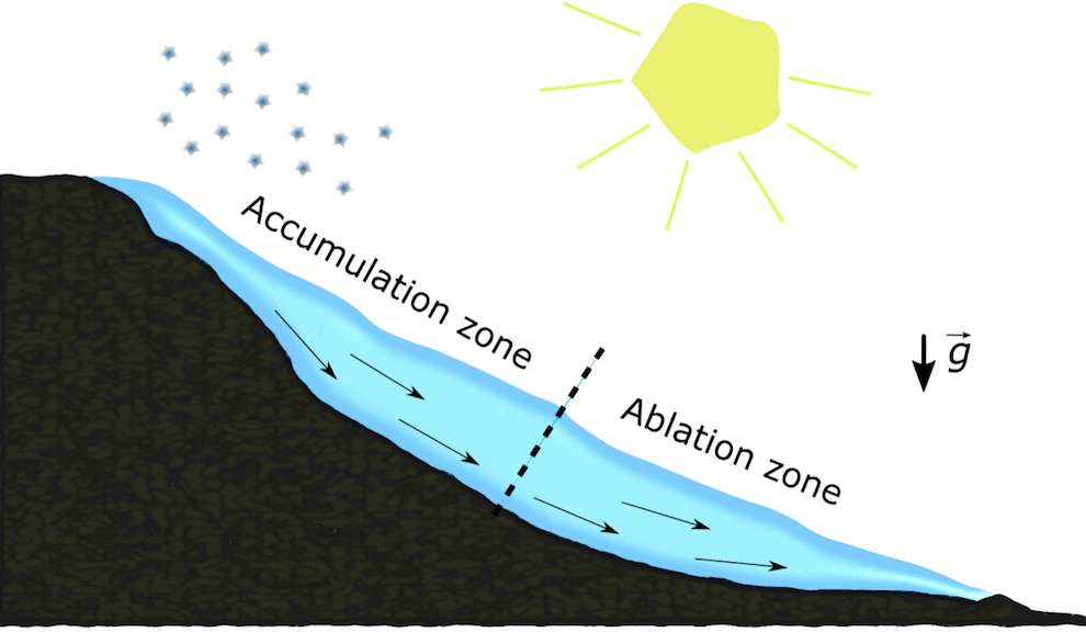
Sketch of a typical mountain glacier.
Thus, we have a dynamical process for the ice, even at steady state (when the snow fall exactly compensates for the melting): creep. This fluid model is a standard Navier-Stokes equation with one simplification: the Stokes (low-Reynolds) approximation, which neglects the advection term. A typical value for the Reynolds number is Re = 10-15, so the assumption undoubtedly holds.
Glen’s Flow Law
The simulation of viscous flow generally assumes a linear relationship between stress and strain. This assumption describes a Newtonian fluid. Many fluids are, indeed, Newtonian in their standard condition (e.g., water and air). However, many fluids exhibit a variation of their viscosity when submitted to shearing. A slightly more general approach is to use a constitutive law to describe the viscosity \mu as a function of a certain power of the shear rate. Mathematically speaking, it is written \mu = \frac{1}{2}A^{-\frac{1}{n}}\dot{\gamma}^{n-1}, where \dot{\gamma} is the shear rate and is classically defined as the norm of the strain rate tensor D(u)=\frac{1}{2}\left(\nabla u + \nabla u^T\right).
Get more details in these blog posts about non-Newtonian fluids and the non-Newtonian behavior of ketchup.
To completely define the flow law, two parameters need to be evaluated:
- Consistency, m=\frac{1}{2}A^{-1/n}
- Stress exponent, n
In the case of ice, it is common to take n=\frac{1}{3}. However, the viscosity of the ice depends not only on the shear rate but also the temperature and pressure. The consistency is then defined in order to represent these dependencies. A classical way to define the consistency in ice modeling is to use an Arrhenius law (Ref. 1): A(T^{\prime},p)=A_0e^{-Q/RT^{\prime}}, where R is the perfect gas constant and T’ is the temperature relative to the pressure melting point.
Indeed, the pressure dependency is reflected through the shift of the ice’s melting point with pressure (which is lowered with increasing pressure). Using the Clausius-Clapeyron relation, we obtain T^{\prime}=T+\beta p, where \beta=9.8\times 10^{-8} K Pa^{-1} is the Clapeyron constant. The values for A0 and Q are a matter of debate. (Ref. 2)
Viscous Slip
This elegant flow law, established empirically over the years through rigorous lab work, has failed to predict the high velocities observed on real-life glaciers. It took many years to understand what was missing. Consensus was brought about by J. Weertman in the late 1950s with the notion of basal sliding.
At an equation level, the basal sliding law of glaciers is not different from the viscous slip concept introduced by H. Navier a century earlier, based on molecular interaction considerations. However, the physical process behind this law, in the case of ice flow, is still a matter of debate and is not the subject of this post. Let’s just recall that it is written as u_t=\frac{L_s}{\mu}\tau_{nt}, where ut is the velocity of the base; \mu is the viscosity (nonlinear here); \tau_{nt} is the basal traction, or the shear stress at the bedrock; and Ls is called the slip length (Ref. 2). This quantity is crucial in glacier flow modeling, as it accounts for a large part of the mass flux downstream, adds up to the flowing movement, and represents a behavior similar to a rigid movement.
Modeling the Flow of Ice: A Real-World Example
The Mer de Glace, which translates to “Sea of Ice”, is a mountain glacier located in the Mont Blanc massif in the French Alps above the Chamonix Valley. Considered the largest glacier in France, it has been widely observed and monitored because of its considerable moving speed for a valley glacier (around 100 meters per year) and its significant retreat and decrease in size in the past 80 years. Studies show an average loss of 5 meters per year in thickness and 30 meters per year in length.
Below (right) is a sketch of a geometry for a valley glacier, set up using COMSOL Multiphysics and the CAD geometric kernel (available with the CAD Import Module). The geometry approximately mimics the measurements and visuals of the Mer de Glace (left).
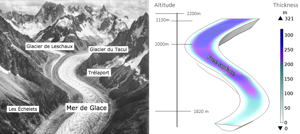
Left: Aerial photo of the Mer de Glace in 1909. Image in the public domain, via Wikimedia Commons. (Annotations added by the author.) Right: Model geometry, colored by thickness.
Let’s simulate the nonisothermal flow of the ice mass downslope, under its own weight and subject to basal sliding.
In terms of fluid, the inflow and outflow boundary conditions are the normal constraints, corresponding to the applied pressure of the ice, which is not included in the domain. It simply corresponds to an assigned hydrostatic (or cryostatic) pressure. The upstream boundary weighs on the domain, thus contributing to a streamwise velocity, while the downstream boundary resists to the flow. The surface of the glacier is a free surface.
In terms of heat transfer, the surface is considered to be at an ambient temperature. The boundary in contact with the bedrock is normally subject to a geothermal heat flux, which could be modeled as a boundary condition. However, since such a value is spatially varying and generally unknown, a temperature is imposed in the present case. This way, we ensure that the ice remains at a temperature below 0°C, thus avoiding the phase change and latent heat flux contribution. It is worth noting that this aspect could be taken into account using a Material with Phase Change interface. Heat is allowed to enter and leave the domain at the inflow and outflow boundaries.
An extruded mesh is used that is consistent with the aspect ratio of the geometry.
The external weather conditions are an important input data for geophysical simulations. Accessing the ASHRAE 2017 database directly through the Heat Transfer interface, we can import the average external temperature and wind velocities at a given time of the year for more than 6000 weather stations all over the world. Here, we use the data from the Grand Saint Bernard station in the Swiss Alps, located at 16 km of the Mer de Glace, around at the same altitude on the first of February at noon. The ambient temperature is imposed at the glacier surface and the wind velocities are used to simulate a convective heat flux at the surface.
Simulation Results and Discussion
First, we run the simulation without basal sliding to see how much the viscous flow contributes to the observed velocities of the glacier. The results are expected to be around 120 meters per year at the top of the glacier and 90 meters per year at the end of the glacier.
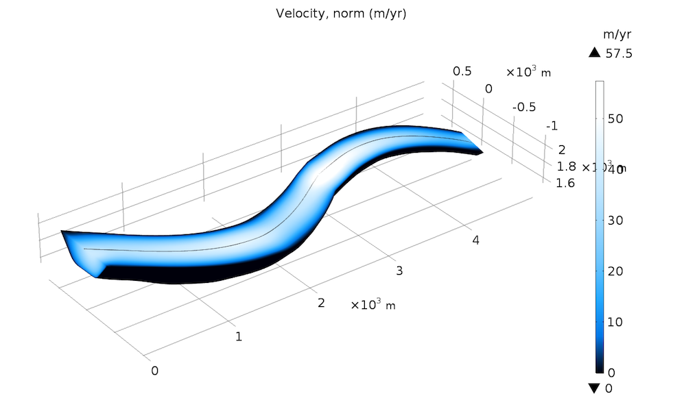
As we can see on the left-hand side of the plot, solely based on the viscous law described here, we get only 50% of the expected velocity.
We can introduce a viscous slip with a slip length Ls = 250 m and run the simulation again. Below, we plot the velocity at the surface along the central flowline of the glacier for both cases.
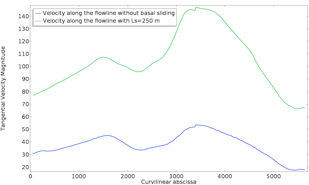
Now the velocity is globally much higher and better matches the expected magnitude. It is interesting to note that the viscous sliding does not only introduce a pure shift of the velocities. Indeed, as a function of the nonlinear viscosity, it adds a nonlinear contribution, thus it is not purely rigid. With this value for the slip length, the sliding contributes to around 60% of the velocity at the surface.
Next, let’s move on to the results about the effect of temperature on the ice flow, which is an important coupling in the context of recent climate change studies. To quantify the effect of global warming on the glacier, let’s consider the following experiment. According to data, the temperature has been globally stable between 1940 and 1970, so we can assume that the glacier reached a steady state during this period. Measurements show that the global average temperature has increased by around 1 degree over 50 years. We can thereby simulate the transient flow of ice over these 50 years with the average temperature steadily increasing for a total of 1 degree.
To see the effect of this change in temperature, we can plot the evolution of the total mass outflux, in megatons per year, at the surface and downstream boundary
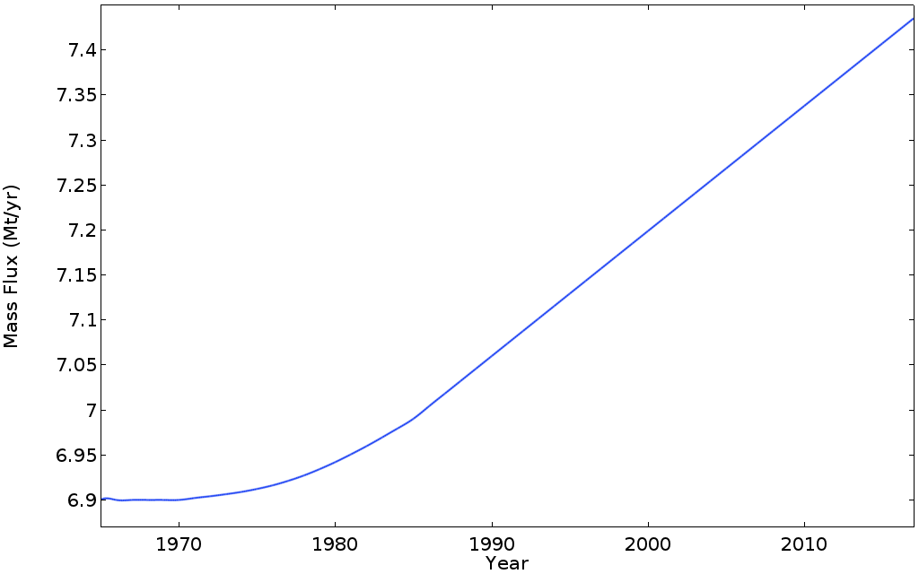
It’s interesting to observe the delay between the beginning of the temperature increase and the glacier response. The linear temperature increase starts in 1970 and the linearly increasing mass flux starts around 1985. Between 1970 and 1985, the acceleration of mass loss slowly increases until it reaches a steady value of approximately 13 kilotons per year square. This delay is mainly due to the time for a temperature change at the surface to propagate through the whole glacier (and thus increase the average temperature in the whole bulk). As a result, the output mass flux is increased by around 10% during this period, leading to a net extra ice loss of 15 megatons over the period (compared to the case where temperature would have remained steady).
Let’s compare our results with the data about the Mer de Glace discussed earlier. If the glacier decreases in thickness by 5 meters per year for our domain (5500 meters long and 600 meters wide in average), we get 15 Mt/yr of ice loss per year. Even assuming that all of this ice flux will melt at a lower altitude (which is not the case), the 7.5 Mt/yr per year computed for 2017 is much smaller than the real mass loss that the Mer de Glace has undergone in past decades. This is because the simulation does not take into account the negative surface mass balance (the accumulation of snow minus the melting of ice at the surface).
Surface mass balance, in terms of modeling, is a data input and itself the product of complicated physics. As an example, hotter summers have a very strong effect on glaciers, because the small amount of snow that normally falls in the summer acts as a shield against solar radiation, thereby protecting the glacier from a large part of summer melting. If the summer snowfall does not occur, the melting is then much greater. This extra melting results in large infiltrations of liquid water through crevasses, which eventually form a subglacial hydrological network that plays a significant role in the basal slipperiness, mostly via the lubrication of the ice-bedrock interface and the water pressure “lifting” the glacier.
The fact that the simulation is performed for a given geometry of the glacier, neglecting the evolution of the geometry through the surface mass balance and dynamics, is also important, since the geometry affects the dynamics.
Concluding Thoughts on Modeling the Flow of Ice
This blog post has presented the setup and solution of a simple glacier flow model with COMSOL Multiphysics. The COMSOL® software offers specialized functionality for most problems involved in such modeling scenarios. The main limitation here, and in glaciology in general, is the data; typically, the topographical data, basal slip length, surface mass balance, accumulation, and melting.
In an upcoming blog post, we will demonstrate how to get the most out of glacier simulations using sensitivity analysis and data assimilation through the Optimization Module. Stay tuned!
Editor’s note, 8/27/18: The second part in this blog series, “How to Analyze a Glacier via Gradient-Based Optimization“, is now live.
Next Step
References
- Climate Change 2013: The Physical Science Basis. Contribution of Working Group I to the Fifth Assessment Report of the Intergovernmental Panel on Climate Change, T.F. Stocker et al. (eds.), Cambridge University Press, 2013.
- R. Greve and H. Blatter, “Dynamics of Ice Sheets and Glaciers,” Springer, 2009.


Comments (2)
KHALIL RAHMAN
January 26, 2021Can i get this model file ?
Mingdong Wei
August 14, 2022Dear Mr. Nathan Martin,
You have done a very good job! I am a beginner in COMSOL and interested in this modeling. Could you please send me the mph file? Thanks!
My email address is weimingdong@163.com