

In a previous blog post, we discussed simulating focused laser beams for holographic data storage. In a more specific example, an electromagnetic wave focused by a Fourier lens is given by Fourier transforming the electromagnetic field amplitude at the lens entrance. Let’s see how to perform this integral type of preprocessing and postprocessing in COMSOL Multiphysics with a Fraunhofer diffraction example.
Understanding Fourier Transformation with a Fraunhofer Diffraction Example
The ability to implement the Fourier transformation in a simulation is a useful functionality for a variety of applications. Besides Fourier optics, we use Fourier transformation in Fraunhofer diffraction theory, signal processing for frequency pattern extraction, and image processing for noise reduction and filtering.
In this example, we calculate an image of the light from a traffic light passing through a mesh curtain, shown below. To simplify the model, we assume the electric field of the lights is a plane wave of uniform intensity; for instance, 1 V/m. Let the mesh geometry be measured by the local coordinates x and y in a plane perpendicular to the direction of the light propagation, and let the image pattern be measured by the local coordinates u and v near the eye in a plane parallel to the mesh plane.
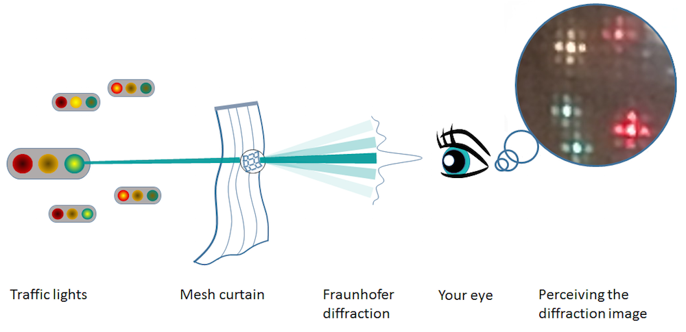
A Fraunhofer diffraction pattern as a Fourier transform of a square aperture in a mesh curtain.
According to the Fraunhofer diffraction theory, then, we can calculate the image above simply by Fourier transforming the light transmission function, which is a periodic rectangular function if the mesh is square. Let’s consider a simplified case of a single mesh whose transmission function is a single rectangular function. We will discuss the case of a periodic transmission function later on.
We are interested in the light hitting one square of the mesh and getting diffracted by the sharp edges of the fabric while transmitting in the center of the mesh. In this case, the light transmission function is described by a 2D rectangular function. By implementing a Fourier transformation into a COMSOL Multiphysics simulation, we can more fully understand this process.
Utilizing Data Sets in COMSOL Multiphysics
In order to learn how to implement Fourier transformation, let’s first discuss the concept of data sets, or multidimensional matrices that store numbers. There are two possible types of data sets in COMSOL Multiphysics: Solution and Grid. For any computation, the COMSOL software creates a data set, which is placed under the Results > Data Sets node.
The Solution data set consists of an unstructured grid and is used to store solution data. To make use of this data set, we specify the data to which each column and row corresponds. If we specify Solution 1 (sol1), the matrix dimension corresponds to that of the model in Study 1. If it is a time-dependent problem, for example, the data set has a three-dimensional array, which may be written as T(i,j,k) with i=1,\cdots, N_t, \ j=1, \cdots, N_n, \ k = 1, \cdots, N_s . Here, N_t is the number of stored time steps, N_n is the number of nodes, and N_s is the number of the space dimension. Similarly, the data set for a time-dependent parametric study consists of a 4D array. Again, note that the spatial data (other than the time and parameter data) links with the nodal position on the mesh, not necessarily on the regular grid.
On the other hand, the Grid data set is equipped with a regular grid and is provided for functions and all other general purpose uses. All numbers stored in the Grid data set link to the grid defined in the Settings window. This data set is automatically created when a function is defined in the Definition node and by clicking on Create Plot. This creates a 1D Grid data set in the Data Sets node.
You also need to specify the range and the resolution of your independent variables. By default, the resolution for a 1D Grid data set is set to 1000. If the independent variable (i.e., x) ranges from 0 to 1, the Grid data set prepares data series of 0, 0.001, 0.002, …, 0.999, and 1. The default resolution is 100 for 2D and 30 for 3D. For Fourier transformation, we use the Grid data set. We can also use this data set as an independent tool for our calculation, as it does not point to a solution.
Implementing the Fourier Transformation
To begin our simulation, let’s define the built-in 1D rectangular function, as shown in the image below.
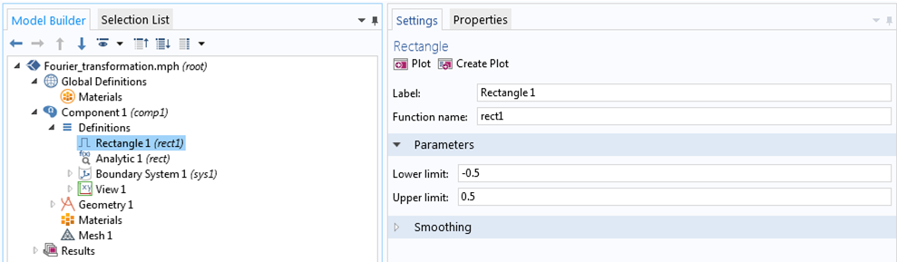
Defining the built-in 1D rectangular function.
Then, we click on the Create Plot button in the Settings window to create a separate 1D plot group in the Results node.
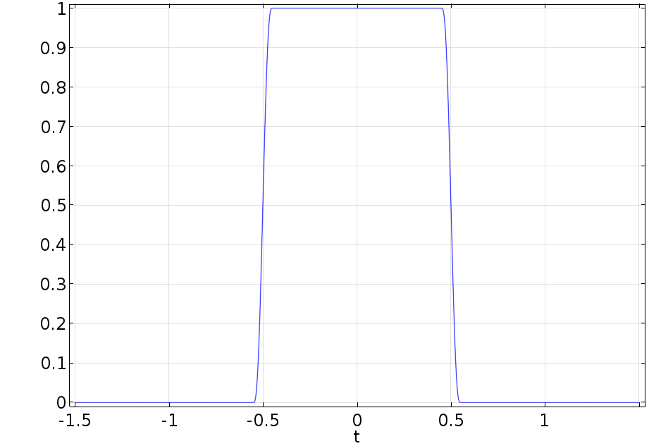
A plot of the built-in 1D rectangular function.
Let’s look at the Settings window of the plot. We expand the 1D Plot Group 1 node and click on Line Graph 1 to see the data set pointing to Grid 1D. In the Grid 1D node settings, we see that the data set is associated with a function rect1.

Settings for the built-in 1D rectangular function.
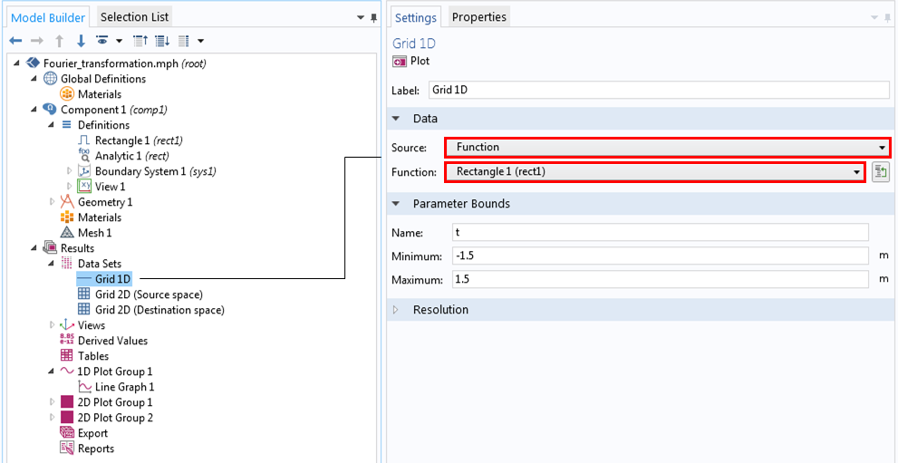
Settings for the 1D Grid data set.
We can create a 2D rectangular function by defining an analytic function in the Definitions node as rect1(x)*rect1(y). For learning purposes, we will create and define a 2D Grid data set and plot it manually instead of automatically. The results are shown in the following series of images.
In the Grid 2D settings, we choose All for Function because the 2D rectangular function uses another function, rect1. We also assign x and y as independent variables, which we previously defined as the curtain’s local coordinates, and set the resolution to 64 for quicker testing. To plot our results, we choose the 2D grid data, renamed to Grid 2D (source space), for the data set in the Plot Group settings window.
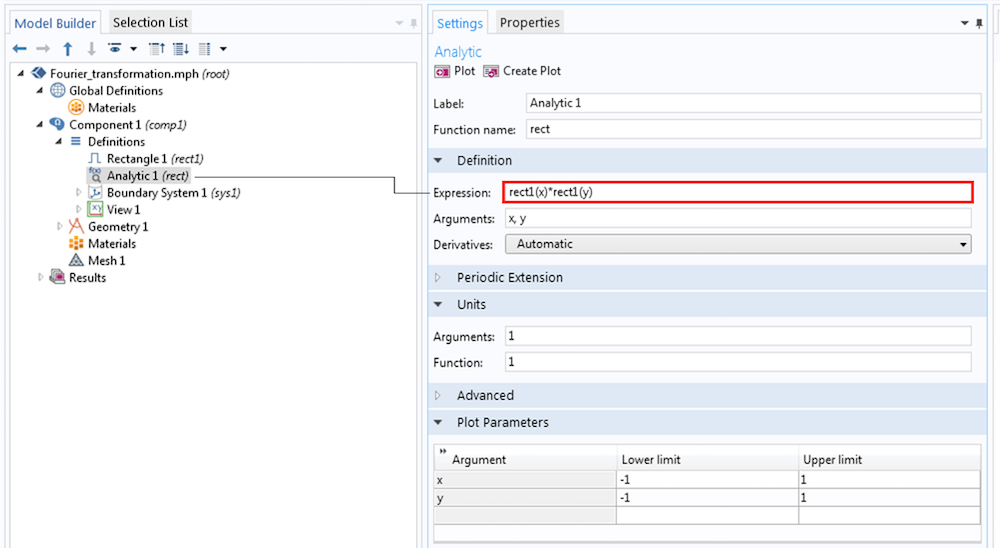
Defining the function in the Grid 2D settings.
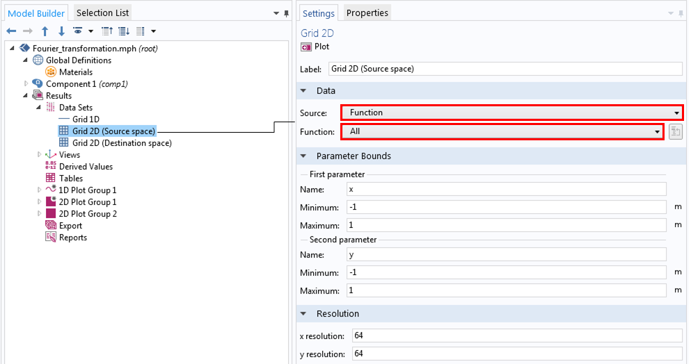
Creating and defining a 2D data set.
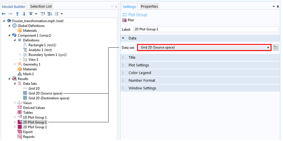
Setting the 2D plot group for the 2D rectangular function.
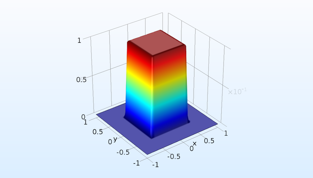
A 2D plot of the 2D rectangular function.
Now, let’s implement a Fourier transform of this function by calculating:
Here, u and v represent the destination space (Fourier/frequency space) independent variables, as we previously discussed.
Since we already created a 2D data set for x and y, now we can create a Grid 2D data set, renamed to Grid 2D (Destination space), for u and v (shown below). We choose Function from Source and All from Function because the rect function calls the rect1 function as well. We can change the resolution to 64 here, as we did for the 2D data set, for quicker calculation.
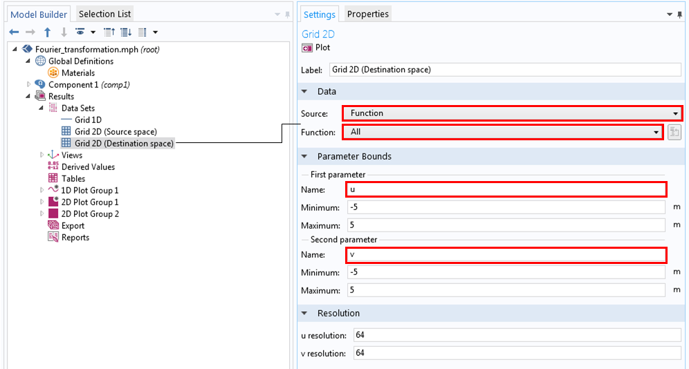
Settings for the Grid 2D data set for the Fourier space.
Now, we are at the stage in our simulation where we can type in the equations by using the integrate operator.
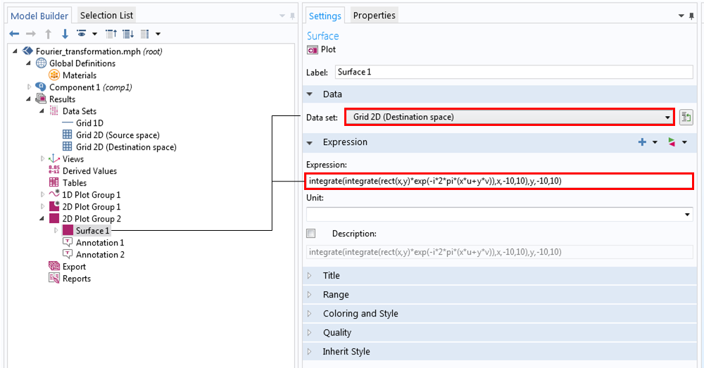
Entering the equation for the Fourier transform of the 2D rectangular function.
We finally obtain the resulting Fourier transform, as shown in the figure below. Compare this (more accurately, the square of this) to each twinkling colored light in the photograph of the mesh curtain. In practice, this image hasn’t been truly seen yet. To calculate the image on its final destination, the retina of the eye, we would need to implement the Fourier transformation one more time.
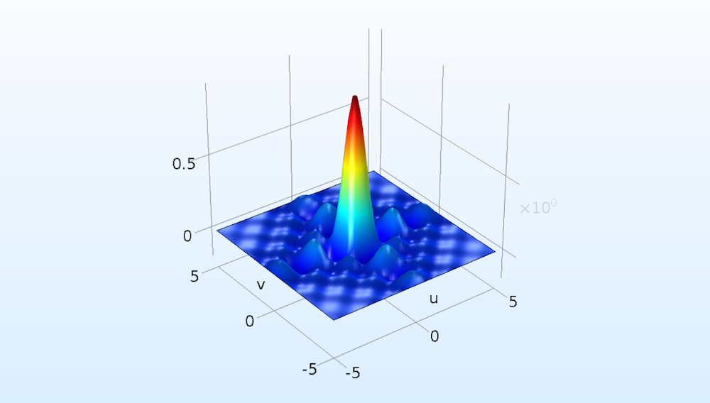
The Fourier transform of the 2D rectangular function.
Concluding Remarks on Fourier Transformation
In COMSOL Multiphysics, you can use the data set feature and integrate operator as a convenient standalone calculation tool and a preprocessing and postprocessing tool before or after your main computation. Note that the Fourier transformation discussed here is not the discrete Fourier transformation (FFT). We still use discrete math, but we carry out the integration numerically by using Simpson’s rule. This function is used in the integration operator in COMSOL Multiphysics, while the discrete Fourier transform is formed by the operation of number sequences. As a result, we don’t need to be concerned with the aliasing problem, Fourier space resolution issue, or Fourier space shift issue.
There is more to discuss on this subject, but let’s comment on the two cases that we simplified earlier. We calculated for a single mesh. In practice, the mesh curtain is made of a finite number of periodic square openings. It sounds like we have to redo our calculation for the periodic case, but fortunately, the end result differs only by an envelope function of the periodicity. For details, Hecht’s Optics outlines this topic very well.
The second simplification was that we assumed a sharp rectangular function for the mesh transmission function. In COMSOL Multiphysics, all functions other than the user-defined functions are smoothed to some extent for numerical stability and accuracy reasons. You may have noticed that our rectangular function had small slopes. This may be a complication rather than a simplification because the simplest case is a rectangular function with no slopes and we used a smoothed rectangular function instead of a sharp one.
The Fourier transforms of the two extreme cases are known; i.e., a rectangular function with no slopes is transformed to a sinc function (sin(x)/x) and a Gaussian function to another Gaussian function. A sinc function has ripples around the center representing a diffraction effect, while a Gaussian function decays without any ripples. Our smoothed rectangular function is somewhere between these two extremes, so its Fourier transform is also somewhere between a sinc function and a Gaussian function. As we previously mentioned, the curtain fabric can’t have sharp edges, so our results may be more accurate for this example case anyway.
Further Reading
- Check out these blog posts about simulating holographic data storage systems:
- Find more information in these introductory books on optics:
- J.W. Goodman, Introduction to Fourier Optics, W. H. Freeman, 2004.
- E. Hecht, Optics, Pearson Education Limited, 2014.


Comments (8)
凯 王
September 10, 2019Hi, this is awesome, anywhere I can downland the Model file? Thanks.
Yosuke Mizuyama
September 10, 2019 COMSOL EmployeeHello 凯 王,
Thank you for reading my blog. This technique is used in some of the application models that we publish, for example, this one: https://www.comsol.com/model/fresnel-lens-46571. In this model, the Fresnel approximation is used, not the Fraunhofer approximation (Fourier transformation). But you can easily modify it for your purpose.
Best regards,
Yosuke
Denis Karpov
August 24, 2020Hi,
proposed approach does not see solution in 2D plot.
Best,
Denis
Yosuke Mizuyama
August 24, 2020 COMSOL EmployeeHi Denis,
Please follow the model called “focusing_lens” in the Application Libraries under the Wave Optics module.
Best regards,
Yosuke
Manish kala
March 22, 2021Thank you Sir for the blog. could you please explain when you are performing integration, why you have used -10, 10.
Yosuke Mizuyama
March 25, 2021 COMSOL EmployeeDear Manish,
Thank you for reading my blog. The integration range is the negative infinity to the positive infinity in the formula. However the rect function has the domain ranges of certain finite sizes (-0.5 <= x <= 0.5 and -0.5 <= y <= 0.5 in this case). So it's a kind of arbitrary what integration ranges you choose as far as it covers the rect function domain range. I hope this helps.
Best regards,
Yosuke
Charles Rambo
January 17, 2024I found this post looking for how to make an FFT of my 2D result. I think this guide could also use some updates; perhaps there have been some changes to COMSOL over the years? My attempt to recreate this breaks at the `rect` function which doesn’t appear to exist. If possible, an explanation of the Grid functions would also help since the documentation is thin and there don’t appear to be any examples for using it with a dataset.
Yosuke Mizuyama
January 23, 2024 COMSOL EmployeeDear Charles,
Thank you for reading my blog. Yes. We did have a new Spatial FFT feature. So we no longer need this manual integration technique unless specially needed. I’m sorry. I don’t understand your problem. The rect function is a built-in function and the gird dataset is automatically created once you create a plot of the function.
Best regards,
Yosuke