

In many applications, loads applied to structures are random in nature. The sampling results of the structural response will differ depending on the data collection time. Although the stress experienced is not always high, the repeated loading and unloading can lead to fatigue. The engineering challenges in these types of applications are defining the stress response to the random load history in the critical points, and predicting fatigue damage. This is simulated with the Cumulative Damage feature in the Fatigue Module, which defines the stress history using the Rainflow counting method and calculates the fatigue damage using the Palmgren-Miner linear damage rule.
Multiple Loads Contribute to Cumulative Damage
Random loads introduce a variety of stresses, with different magnitude, into a structure. It is therefore important to identify overall trends in the stress history. Rainflow cycle counting is a popular method to transfer the variable load history into a discrete stress distribution that is characterized by certain mean stress and stress amplitude. In COMSOL Multiphysics, the stress distribution of the Rainflow counting is visualized in a new plot type, called Matrix Histogram.

Stress distribution based on the Rainflow cycle counting method.
A classic way of obtaining fatigue life is via the S-N curve. It relates the stress amplitude to the number of loading cycles a material can withstand. In variable loading however, the stress amplitude is not constant and, instead, you must use an alternative model that calculates damage contribution of each cycle. You might use the Palmgren-Miner linear damage rule, a widely used method, to capture this. In the Fatigue Module, the Palmgren-Miner rule processes the stress distribution of the Rainflow counting and relates it to the limiting S-N curve. In order to capture the mean stress effect, so that damage increases with the increasing mean stress, the S-N curve is specified with an argument for the R-value.
Cumulative Damage Calculation Based on Generalized Loads
The fatigue analysis consists of two steps. First, you calculate the structural response of a load cycle. Next, you perform a fatigue evaluation. When the number of load events is large in a random load analysis, the simulation of the load cycle is time consuming, but the calculation time can be greatly reduced if the nonlinear effects are not present in the simulation. In that case, the stress cycle can be prescribed with help of superposition. This is selectable with the Generalized loads analysis type in the Cumulative Damage feature. There, the load cycle is not prescribed load-step by load-step, but instead the history of an external load is decomposed into few generalized loads with corresponding load histories.

The external load simulated using three generalized loads and corresponding time histories.
The Cumulative Damage calculation, based on the generalized loads, can be summarized in following steps:
- Define generalized loads
- Prescribe generalized loads in a structural study
- Compute structural response to generalized loads
- Define load histories for all generalized loads
- Prescribe load histories to corresponding generalized loads
- Compute fatigue analysis
The first three steps are done in a structural prestudy, while the last three are done in a fatigue study.
Fatigue Modeling Examples
I’d like to share two examples of simulating Cumulative Damage, with you. Both can be found in the Fatigue Module. In one of the examples, the load cycle is prescribed step-by-step, and in the other one, superposition is used via the Generalized loads option.
The “Frame with Cutout” example uses the Generalized loads option. Here, the fatigue response to 1,000 load events is simulated. The total computation time with the Generalized loads option is 8 minutes, while the load event by load event calculation takes 1.5 minutes for each load event, thus the total load cycle would require a full day of computation time. Moreover, large amount of data needs to be saved in order to be processed by the fatigue study. With the Generalized loads option you don’t need to spend this much time on your computations.
The model “Cycle Counting in Fatigue Analysis — Benchmark” compares results of the Rainflow counting against an ASTM standard. The results based on the Palmgren-Miner are compared against hand calculations.
If you’re interested in learning more about fatigue modeling, tune into our Fatigue Modeling with COMSOL webinar on July 30th, 2013.

Comments (0)